Watersheds and flow parameters. Watersheds (also called basins or catchments) are defined as the areas draining into a single point. They are a suitable choice as landscape units for land use and natural resource management. Output of such units, in terms of water discharge, sediment, and pollutant loads can be relatively easily monitored, providing a quantified measure of impact of land management actions.

Because each point of landscape has a watershed associated with it (it can be anything from the point itself for a peak to hundreds of square miles for outlets of big rivers), we need to select a suitable size for our watershed management units. For our study area, a 50000 grid cells watershed size can be used as a threshold parameter for r.watershed. We also compute a flow accumulation map and a drainage map, as they may be needed as inputs for models:

The report shows that our basins have areas from 15 to 153 acres. We have used d.what.rast to find the number of the watershed that will be the focus of our more detailed study (it has category number 6) and according to our report table it has 62.81 acres. We can create a vector representation of watershed boundaries (Figure 12.5) using r.poly so that we can overlay them over other data such as imagery, or transfer them to GPS to guide mapping activities:

To view the accumulation map, you need to create a non-linear color table for accum.6 as explained in the previous Section 12.1, or display only the cells with high values, for example:

d.rast accum.6 cat=10000-400000

Remember that r.watershed uses the D8 algorithm, so it is not suitable for hillslope flow pattern (Figure 12.5 a, b). It flows through all depressions (unless they are explicitly given as input), so the stream network will be fully connected and drain into the outlet. We can get the coordinates for the watershed outlets using d.what.rast:

d.rast basin.6 d.vect lw hydro d.what.rast

2096054.56(E) 721547.96(N) basin.6 in lakewheeler hm (6)

2097854.97(E) 721043.84(N) basin.6 in lakewheeler hm (4)

and then input the outlet coordinates into GPS for evaluation of the suitability of these locations for monitoring directly in the field. It is highly probable that the exact points derived from the watershed map wont be ideal for monitoring and new locations may be selected. It is then necessary to derive the modified watershed boundaries for the exact locations of the monitoring stations using r.water.outlet. In our study area, we are installing two monitoring stations: one at the point A (Figure 12.5) near the road above a constructed wetland (2095700.00, 722600.00) and one at the point B which is the outlet for our entire study area. The first station is far from the outlet of the watershed number 6; therefore, we need to delineate a new one. Because the stream.6 map layer does not show a stream in our subarea (the threshold for streams is higher, as we can see by displaying lw hydro vector map over stream.6), we need to use the accumulation map to compare the field monitoring location with the concentrated flow defining the outlet. We find that it is shifted by a few meters and there are only few cells upflow from this point. Also at 6 ft resolution, the flow from r.watershed is split into many parallel lines (Figure 12.5 a), therefore we need to decrease resolution to get a single, clearly defined outlet. We can then find new coordinates for outlet using d.what.rast and define a new watershed. The entire procedure is as follows:

g.region res=20 -p

r.watershed elev=el.6tlO accum=accum.20 basin=basin.20 \

threshold=2000 drainage=drain.20 stream=stream.20 r.colors accum.20 rast=accum.6 d.what.rast [. . .]

20 9564 8.7 995692 8(E) 722 620.03377117(N) [...]

r.water.outlet drainage=drain.20 basin=basin.A20 \

east=2095648 north=722620

d.rast basin.A20 g.region res=6

r.poly -1 basin.A20 out=basin.A20 d.vect basin.A20 col=blac)c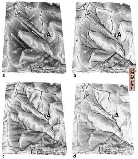

Figure 12.5. Flow accumulation maps based on a) D8 method (r.watershed) 6 ft resolution, b) D8 method (r.watershed), 20 ft resolution, c) vector-grid (D-infinite, r.flow) 6 ft resolution, d) multiple directions flow (r.topidx). Watershed boundaries as derived from r.watershed and r.water.outlet for the monitoring station A are shown as vector lines draped over the DEM

The flow accumulation map generated at 20 ft resolution has better defined concentrated flow areas, making the delineation of the watershed above the monitoring station A feasible (Figure 12.5 b). Note that for some hydrologic and pollutant transport models, we could further divide the study area into