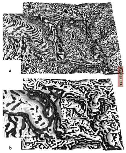Figure 12.3. Interpolating DEM from contours: profile curvature displayed with input contours a) tension is too high and the pattern of curvature follows contours, b) with lower tension the pattern disappears

For some applications it is useful to create a DEM with buildings. We can compute it using the building footprints which are available as vector data. First, we need to transform them to raster and then we add their average height, in our case 20 ft, to the DEM:

v.to.rast lw buildings out=buildings d.rast el.etlO d.rast -o buildings r.null buildings null=0

r.mapcalc elevbldg.6=if(buildings > 0, el.6tl0+20, el.6tl0) r.mapcalc elevbldgco.6=if(buildings > 0, -1, el.6tl0) r.colors elevbldgco.6 rast=el.6tl0

nviz elevbldg.6 col=elevbldgco.6 vector=lw roads,lw hydro

Note that we had to convert NULLs in the buildings map to zeroes first because NULLs override any other value when used in r.mapcalc expressions (see Section 5.2). We have also created an additional raster to be used for color and displayed it together with roads and streams in 3D using nviz (Figure 12.4). The surface has the typical elevation color scheme with buildings displayed in white with grey shades. You can adjust the z-exaggeration and light to enhance the 3D perception and save your view as a PPM, TIFF or RGB image (see Chapter 8).

Topographic analysis. Topography has a profound influence on fluxes in landscapes and is often a major factor in decisions related to land use. Therefore map layers representing watershed boundaries and topographic parameters (see Section 5.4) are used as the basis for selection of land management units,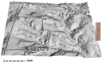

Figure 12.4. High resolution DEM interpolated from 2 ft contours with buildings viewed in nviz. Our practice area is in the west section

placement of monitoring equipment, evaluation of suitability of the current land use for existing topographic conditions and a number of other issues.

Local (point) topographic parameters. A number of parameters describing the geometry of the terrain surface are needed as inputs for land use suitability analysis and modeling of various processes. These parameters represent measures of change in elevation (gradient) and measures of rate of this change (curvatures) and are usually expressed as the following parameters (see also Section 5.4.5 and the exact mathematical definitions and equations in the Appendix B.3):

slope (steepest slope angle, magnitude of gradient);

aspect (slope orientation, direction of gradient, steepest slope direction, direction of flow);

profile curvature (curvature in the direction of the steepest slope - perpendicular to contour lines, convex curvature leads to accelerated and concave to decelerated flow);

tangential curvature (curvature in the direction of contour tangent - perpendicular to the steepest slope direction, convex curvature leads to dispersal and concave to convergent flow).

It is possible to define a number of additional parameters (see, for example the module r.param.scale), however, for most applications only slope and aspect is needed.

We have already computed these parameters simultaneously with interpolation using v.surf.rst, and we have used the profile curvature to look for artificial patterns in the DEM (Figure 12.3). We have also used r.slope.aspect to derive slope and aspect from the USGS NED data to evaluate potential problems in this DEM (see the relevant paragraph above).

Because the landscape processes have multiscale character and different processes are dominant at different scales, it is sometimes useful to extract topographic features and patterns at different levels of detail. In s.surf.rst or v.surf.rst, this can be achieved by changing tension and smoothing (lower tension and higher smoothing produces smoother topography with curvatures representing main features, higher tension captures more detail and smaller features, see Section 7.3 as well as the Figure 12.3). We can also use r.param.scale, which has additional options to extract the main topographic features, peaks, ridges, passes, channels, pits and planes and compute a number of additional parameters.

Learn more about topographic analysis in the book by Wilson and Gallant, 2000, and publications by Wood, 1996, Mitasova and Hofierka, 1993, and Moore and Burch, 1986.