of this map for each attribute and then copy its vector category file to the new raster category file (see Section 4.2.1 and Section 5.1 for more details about categories). You can check which attributes were included with the soil data layer by listing the files in the vector categories subdirectory dig cats in the related MAPSET directory: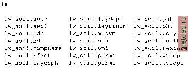

The attributes are described in the NRCS documentation. If you plan to do substantial work with multiattribute data, it is worth considering the link with databases such as PostgreSQL or another DBMS linked through the ODBC interface. This functionality has been substantially improved in GRASS 5.7, the development version. Here, however, we will work only with GRASS 5.3 tools.

To create a raster map layer with the names of soils using the category file lw soil.musym, we run (from within the appropriate MAPSET directory):

g.copy rast=lw soil.6,lw soil.musym cp ./dig cats/lw soil.musym ./cats d.rast lw soil.musym r.report lw soil.musym unit=a,p

A raster map layer for the K factor can be generated from lw soil. kf act file in a similar way: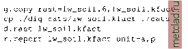

If we need additional raster maps of soil properties, we just create a copy of the raster lw soil. 6 with the appropriate name and copy the relevant category file to the raster cats directory as shown above.

Land cover. Land cover data are usually derived from satellite or aerial imagery. For our area, 50 ft (16 m) resolution Land use/Land cover (LULC) data and 90 ft (30 m) resolution National Land Cover data are available. Both are derived from satellite imagery for regional scale studies. They do not have the

level of detail needed for local planning, for example, the individual fields or service roads are not represented.

To get more detailed information about the land cover, we downloaded and imported the 1 ft resolution Infrared Digital Orthophoto Quarter Quadrangles (IR-DOQQ, from the Wake county GIS, see URL in Endnotes). The imported images can be used to digitize the individual fields, roads, ponds and other features and to create a high resolution land use map layer. We have imported such a land use map as polygon vector data; you can display it and transform it to a raster as follows (remember that you need to be in an appropriate MAPSET directory to copy the category files):

d.vect lw landcov

v.to.rast lw landcov out=lw landcov d.rast lw landcov

g.copy rast=lw landcov,lw landcov.type id

cp ./dig cats/lw landcov.type id ./cats/lw landcov.type id d.rast lw landcov.type id

r.mapcalc lw landcov.type=int{@lw landcov.type id) d.rast lw landcov.type

We have created two raster maps for land cover. The values stored in lw landcov.type id are unique category numbers for each field, with category labels representing a number associated with a particular land use. This map can be used for creating new management scenarios by assigning different types of crops or land use to the individual fields. Because many fields have the same land use type, we have created a simplified raster map lw landcov.type using r.mapcalc. In this map, the values represent the land use type; we assign them description as a category label using r.support. You can check the land use categories and their area as follows: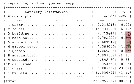

12.2.2 Deriving new map layers

The basic data sets provide foundation for the study of landscape, its properties, and spatial relations between its features. To analyze the landscape and its processes, we need to derive additional map layers which provide information about the landscape properties in the form needed for models and decision making.

Computing the DEM and basic topographic parameters. While the contour data are a standard for representation of topography on paper maps, spatial analysis and modeling can be done more efficiently with a raster DEM. To compute the raster DEM we can transform the points defining the contour lines to sites and use s. surf.rst. It allows us to simultaneously compute the topographic parameters slope, aspect and curvatures that we will need later both for planning and modeling. First we set the region to our study area, defined by the soil map layer, and the resolution to 6 ft, which is enough to capture the roads and dams. Then we can try to run s.surf.rst with the default parameters and include the profile curvature in the output. As we have mentioned in the Section 6.4.3, interpolation from contours often leads to a surface with waves along contours. This can result, for example, in a false pattern of erosion and deposition (see Mitas and Mitasova, 1999) and it is useful to check this by displaying profile curvature along with contours as shown in the Figure 12.3.

g.region res=6 vect=lw soil -p v.to.sites -ad lw contour out=lw contour s.info lw contour

s.surf.rst lw contour elev=elev.6 pcu=pcurv.6 & d.rast pcurv.6 d.vect lw contour

As you can see, for this data set, the tension is too high and the curvatures follow the pattern of contours (Figure 12.3). In some locations, we can even see the triangles which were used to derive the contours. The geometry of the resulting surface thus reflects the geometry implied by the distribution of data points rather than real terrain. To minimize this bias we can lower the tension, reduce the density of points, and introduce slightly higher smoothing:

s.surf.rst lw contour elev=el.6tlO slope=sl.6tlO asp=as.6tl0 \ pcu=pc.6tlO tcu=tc.6tl0 dmin=9 ten=10 smo=0.8 &

d.rast pc.6tl0 d.vect lw contour nviz el.etlO

We will lose some detail, but we will also reduce the artificial patterns, as you can see by overlaying the profile curvature with contours. We can explore the results by displaying the DEM in nviz and draping the computed topographic parameters and contours over it.