lon 0 lat 0 lat l lat 2

7 9dw 33d45n 36dl0n 34d20n

PROJ UNITS file: unit: foot

units: feet meters: 0.3048000000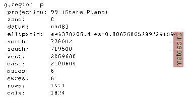

Many counties in US still use feet for their GIS, so to minimize the need for data projection, the database was set up in the State Plane NAD83 coordinate system with feet as units. This will allow us to discuss some issues related to the use of units different from meters in GRASS. Note that in GRASS 5.3, information about the horizontal datum is included in the PRO J INFO file.

For our project, we will need the base map data such as elevation, surface water (streams and lakes), roads, railroads, and land use/land cover. We may also need thematic map layers important for land management, such as soils or climate data. By running the g.list command we can find out which data layers are available and then evaluate whether they are suitable for our project. We will now look at some of the given data in more detail.

Elevation. First, we explore the possibility of using the elevation data elev.90ft from the USGS National Elevation Data set (NED) which merges the best elevation data available into a seamless, approximately 90 ft (30 m) resolution raster format. The data were downloaded from the USGS NED web site in geographic coordinates and projected into the State Plane, feet coordinate system. To evaluate the data quality, we compute and display the slope and aspect and then view the data in 3D using nviz:

g.region rast=elev.90ft -p

r.slope.aspect elev.90ft slo=slope.90ft asp=aspect.90ft \ zfac=0.3048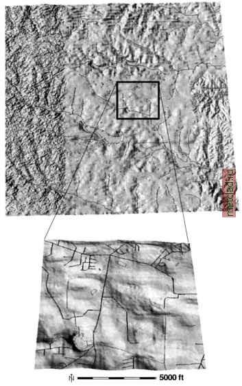

Figure 12.2. Sample from the USGS seamless National Elevation Data set (elevation map with vector roads overlayed) showing insufficient resolution in our study area and overall variable quality, revealed when viewing in nviz

d.rast aspect.90ft d.rast slope.90ft nviz elev.90ft

When computing slope in a LOCATION with units set to feet, it is important to use zfac=0.3048 to obtain the correct values of slope. GRASS internally transforms the distance to meters and it is the users responsibility to transform the elevation values to meters, too; otherwise, the slopes will be severely exaggerated. The slope and aspect maps, as well as Figure 12.2 created with nviz, show that in our study area, the NED elevation model has low resolution, and within the region it has uneven quality. While this elevation data would be appropriate for a regional scale study, they are not suitable for local land management.

Wake county provides topographic data in the form of 2 ft contours as vector data in ESRI SHAPE and E00 format upon request. We have acquired the data and included them in the provided data set. To view the contours run:

g.region vect=lw contour -p d.vect lw contour col=brown

The contours provide a detailed description of topography; however, for most of our applications, we will need elevation data as a raster DEM. We will create it using spatial interpolation in the next Section 12.2.2.

Recently, LIDAR-based elevation data became available for this area in the form of bare ground point data, 20 ft grid and 50 ft grid with stream enforcement. The data can be downloaded from the North Carolina Flood Mapping Program6.

Roads, buildings, streams, soils. Additional vector data are line features representing roads, streams and lakes and building footprints. We will display them using d.vect: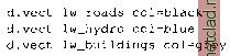

The soil data are available as a polygon map layer. After runningv. support, we transform them to a soil raster map at 6 ft resolution: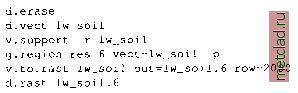

We get a nice map; however, if we run r. report lw soil. 6 we can see that the map includes only polygon numbers. To create raster maps with properties that we will need for modeling and analysis, we have to make a new copy