You can then run the histogram and report:

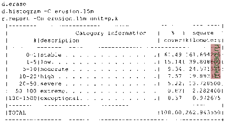The report shows that in spite of the very high topographic erosion risk, most of the Spearfish area is quite stable with over 76% area at relatively low erosion risk. However, there is still about 15% area which has high potential for erosion. You can find where those areas are and what their land use is by creating a land cover map for hot spots using r.mapcalc: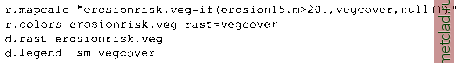

If erosion is above 20 ton/(acre.year), then the raster value from vegetation map layer will be copied to the new raster, all other cells will be assigned the NULL. The result is a land cover map for areas with high erosion risk and NULLs elsewhere. You can see that the forest dramatically lowers the erosion risk making the mountainous area mostly stable, except for areas with rangeland. You can also compute statistics for your erosion.lSm map layer:

r.univar erosion.lSm [. . .]

Number of cells (excluding NULL cells): 1168638 Minimum: 0

Maximum: 699.0562907236

Range: 699.056

Arithmetic mean: 5.02223

Variance: 211.117

Standard deviation: 14.5299

Variation coefficient: 289.311 %

12.2. GIS MODELING FOR LAND MANAGEMENT ()

In this section you will be a GIS expert for a team preparing sustainable land management plan for an experimental farm in Wake county, North Carolina. You will be asked to provide comprehensive geospatial support for your colleagues who will be making decisions and creating plans for this area.

Our study location faces development pressures from the neighboring metropolitan area. At the same time there is a strong support of the current community for preserving open spaces and the rural character of the area. Water from the farm goes to a water reservoir which serves as a backup for drinking water for the neighboring city, making water pollution prevention a key land management issue.

To fulfill this task you propose to do the following:

Build a GIS database for the study area:

search the Internet, contact local agencies to find what data are available;

decide which coordinate system will be used for the core LOCATION used for modeling and analysis;

set up the necessary LOCATION(s), import and project data to common coordinate system;

- evaluate the quality of data, identify missing information and needs for additional mapping and/or monitoring together with other members of the team;

Analyze the data and derive additional map layers needed for the project: create raster DEM from contours, add buildings for 3D view;

While the range of values is extremely high, the mean erosion for this area is relatively low, confirming that the exceptionally high erosion risk applies to only a very small number of grid cells (mostly disturbed areas on steep slopes over 25°). Note that your numbers may be slightly different because of small differences in DEM due to its interpolation from random sites and potential future updates to the Spearfish data set.

To compute a more detailed and up-to-date erosion risk map, you can change your region to the raster map Isfactor.lOm and re-run the computation using the LS factor and C factor based on the new data.

This example demonstrated an application of GRASS for regional scale natural resource management task by assessing erosion risk and identifying critical areas where land use change may be desirable.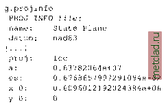

- derive slope, aspect, and curvatures describing the terrain geometry;

- delineate watersheds and flow related parameters; create high resolution land cover map;

Analyze the current land use, identify potential problems and solutions:

- identify areas unsuitable for crop production;

- find suitable locations for selected crops;

- evaluate erosion and sedimentation risks; assess need for conservation measures; evaluate the impact of potential development;

Communicate the results: create maps, views and put data on-line.

While we cannot describe all these tasks in detail, we will show how to do some of them and you can try to find out how to do the ones that sound interesting by yourself.

12.2.1 Building the GIS database

Building the database is usually the most time consuming and sometimes frustrating part of GIS work, no matter what kind of software you use. However, once the data are gathered and nicely integrated in a consistent manner, the work with geospatial data may become quite exciting and rewarding. The task of searching and acquiring the georeferenced data is becoming easier due to the rapid development of WebGIS technology. For example, several data sets needed for this project are available from the Wake county GIS site3. Our study area is covered by tiles 0791 and 0792 that can be accessed directly from the related Map Section.4 We have downloaded the data from the Wake county GIS and other sources, and prepared a ready to use database available from the GRASS Tutorials Web site5 as wake spft new.tar.gz. After downloading and installing it (in a similar way as we did for Spearfish) we can start to explore the data that are available.

First, we need to check the projection, units, and region that have been used for the database: