This page intentionally left blank

g.region -p rast=landcover.30m d.erase

d.rast landcover.30m

d.rast.leg -n landcover.30m

r.recode landcover.30m out=cfactor.30m

> 11:23:0.:0.

> 31:32:0.8:0.8

> 41:41:0.0005:0.0005

> 42:42:0.0008:0.0008

> 43:43:0.0005:0.0005

> 51:71:0.001:0.001

> 81:81:0.01:0.01

> 82:83:0.2:0.2

> 85:85:0.001:0.001

> 91:92:0. :0.

> end

The individual categories are described in more detail in the metadata file provided with the land cover map; therefore, more accurate values of the C factor can be assigned. To get a nice map, we define a special color table: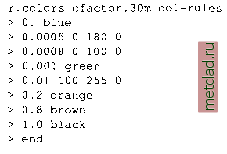

d.rast cfactor.30m

You can compare the new C factor with the one derived from the 100 m resolution vegcover data to appreciate the higher quality of the new data.

12.1.3 Computing and analyzing erosion risk

Finally, we can calculate the erosion risk for the given vegetation cover using r.mapcalc. In the map layers soils.Kfactor, cfactor.lQQm, we use the representation of K factor and C factor as category labels and we have to put at (@) in front of the map name so that r.mapcalc uses the category labels instead of category numbers:

g.region -p rast=lsfactor.15m

r.mapcalc erosion.15m=65. * @soils.Kfactor\

* lsfactor.l5m * @cfactor.100m

The resulting map layer represents soil erosion rate at the center of each grid cell in ton/(acre.year). Note that GRASS has automatically resampled the rasters representing the soils and the C factor from their original resolutions (20 m and 100 m) to 15 m resolution. Because these two map layers represent discrete homogeneous areas, identified by their integer category numbers (and not continuous fields), such resampling is appropriate.

Similarly as for the LS factor, it is useful to define a special color table and categories for the resulting map, while keeping in mind the skewed distribution of erosion rates, with most areas within the low rates range and very few areas in a large interval of high values: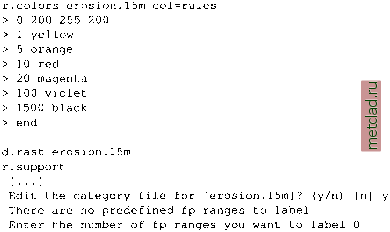

Now type 7 over 0 followed by <ESC><ENTER>, and you will see the category table with floating point ranges all set to zero. Overwrite the zeros with your selected values and add the category labels:

The fp data in map erosion.15m ranges from 0.00 to 699.056291 [erosion.15m] ENTER NEW CATEGORY NAMES FOR THESE CATEGORIES

65.*@soils.Kfactor*Isfactor.15m*@cfactor.100m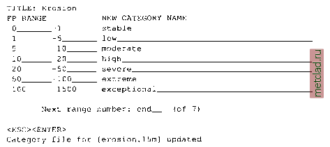