
|
|
|
|
Главная --> Промиздат --> Map principle r.mapcalc Isfactor.30m=l.4*exp(flowacc.30m*30./22.1,0.4)\ *exp(sin(slope.30m)/0.09,1.3) Before displaying the Isfactor.BQm map layer, we assign it a special color table to account for its skewed distribution (similarly to flow accumulation): 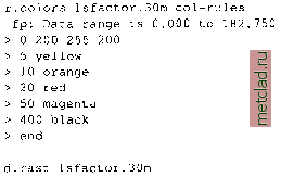 Because this is a floating point map representing a continuous field, the colors smoothly change between the defined color values. The first color is light green, defined as RGB (see Chapter 8). The last black color is defined for a value higher than the maximum LS factor, so that the map color for the highest LS factor is darker magenta. It also makes the color table usable for map layers with a greater range of values than we have in Isfactor.BQm that we will compute later. When we display the map, we can see that we have a substantial area with zero topographic factor for erosion (Figure 12.1). This indicates that the vertical precision the DEM (given as integer values in meters) may not be adequate. Re-interpolation of DEM. We will try to improve the representation of topography by re-interpolating the DEM from 30 m resolution integer z-values to 15 m resolution floating point z-values. While the re-interpolated DEM does not include more information than the original elevation data, its digital representation is improved by removal of the flat areas and steps due to the integer representation, by better description of curved terrain features such as valleys and shoulders through a finer grid. We will use the RST method (see Section 7.3.2, Mitas and Mitasova, 1999) for re-interpolation. Note that this step is not necessary if the DEM already has adequate resolution and precision. We will base the re-interpolation on random points generated from the original integer DEM. First, make sure that the region (extent and resolution) is the same as the original elevation map by running g.region. Then, sample the existing DEM with 100,000 random points (you can use r.info to find the number of cells in your DEM and then choose about 1 point for 2-3 cells): g.region rast=elevation.dem -p r.info elevation.dem r.random elevation.dem nsites=100000 sites out=elev30.sites Next, change the resolution to 15 m and interpolate the newly created sites map layer using s.surf.rst with lowered tension and increased smoothing parameter to reduce the impact of steps and noise in the low elevation areas (see Section 7.3.2 for more details on parameters for spline interpolation). Because we will also need slope angle, we add the computation of topographic parameters to the interpolation. Finally, we add the UNIX & symbol to make it run in the background, because interpolating a 932 x 1266 grid will take some time: g.region -p res=15 s.surf.rst in=elev30.sites elev=elev.15m ten=30 smooth=1.0\ slope=slope.15m aspect=aspect.15m & We can now use this re-interpolated and smoothed DEM to derive a new LS factor: 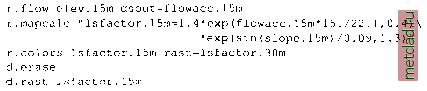 To make the visual comparison with the lsfac.30m easier, we have assigned the new Isfactor.lSm the same color table. Recently, a new 10 m resolution DEM has become available for the Spearfish area; it is included in the data set as elevation.lOm. You can set the region to the new DEM and compute the refined LS factor as follows: g.region -p rast=elevation.10m r.flow elevation.lOm dsout=flowacc.10m r.slope.aspect elevation.lOm slope=slope.10m aspect=aspect.10m r.mapcalc Isfactor.1Om=l.4*exp (flowacc.10m*10./22.1,0.4) \ *exp(sin(slope.10m)/0.09,1.3) r.colors Isfactor.lOm rast=lsfactor.30m d .erase d.rast Isfactor.lOm nviz elevation.lOm col=lsfactor.10m You can see much more detail in the resulting map, especially when displayed in 3D using nviz (Figure 12.1). Noise has been greatly reduced, but there are some waves along contours and local pits, typical for spline interpolation with tension set too high (see Section 7.3). Unfortunately, USGS does not provide details about the method used to create this new product. Comparison of the 10 m, 15 m and 30 m resolution LS factors. The visual comparison of the Isfactor.lOm, Isfactor.lSm, and lsfactor.30m maps indicates that there is a larger extent of areas where LS = 0.0 in the 30 m resolution map than in the 15 m and 10 m resolution result (Figure 12.1). You can run d.rast lsfactor.30m val=0 d.rast Isfactor.lSm val=0 d.rast Isfactor.lOm val=0 to see the difference. To quantify it, we can compare the summary statistics for the results by running r.univar. To make sure that the comparison is correct, we apply MASK so that the NULLs present in Isfactor.BQm (due to the NULLs in the original DEM) are also counted as NULLs in lsfactor.15m and Isfactor.lQm, (see Section 5.1.7 on how to apply a MASK): g.region -p rast = lsfactor . 30m r.mapcalc maskdem=if(elevation.dem,1) g.copy rast=maskdem,MASK r.univar lsfactor.30m [. . .] Number of cells (excluding NULL cells) : 290123 Minimum: 0 Maximum: 182.7502010664 Range: 182.75 Arithmetic mean: 6.90423 Variance: 63.3764 Standard deviation: 7.96093 Variation coefficient: 115.306 % g.region -p rast=lsfactor.15m r.univar ls£actor.l5m [. . .] Number of cells (excluding NULL cells) : 1169268 Minimum: 0 Maximum: 279.8847366021 Range: 279.885 Arithmetic mean: 7.35935 Variance: 61.6206 Standard deviation: 7.84988 Variation coefficient: 106.665 % g.region -p rast=lsfactor.10m r.univar Isfactor.lOm Number of cells (excluding NULL cells): 2626610 Minimum: 0 Maximum: 274.7339156185 Range: 274.734 Arithmetic mean: 7.77852 Variance: 75.6691 Standard deviation: 8.6988 Variation coefficient: 111.831 %
|