Chapter 12

USING GRASS: APPLICATION EXAMPLES

In this chapter, we explain the practical use of GRASS using examples in the area of natural resources. First, we illustrate simple modeling using the Spearfish data set. More complex application is included in the section focused on land use management. To save space, we use the command line mode throughout this chapter; however, the same tasks can be performed by accessing the commands using the TclTk interface or an interactive mode (see Section 3.1.3).

12.1. WORKING WITH DIGITAL ELEVATION MODELS: EROSION RISK ASSESSMENT

In this section, we will use topographic analysis and map algebra to find locations with high erosion rates. To compute simplified erosion risk maps, we can use the widely accepted Universal Soil Loss Equation (USLE), modified for complex terrain (see Mitasova et al., 2001). It is often referred to as

USLE3D or the updated RUSLE3D. The general formulation for both USLE and RUSLE is defined as follows:

A = RKLSCP (12.1)

where A is average annual soil loss in ton/(acre.year)=0.2242kg/(m.year), R is rainfall factor in (hundreds of ft-tonf.in)/(acre.hr.year)=17.02 (MJ.mm)/(ha.hr.year), K is soil erodibility factor in (ton acre.hr)/(hundreds of acre ft-tonf.in)=0.1317(ton.ha.hr)/(ha.MJ.mm), LS is a dimensionless topographic (length-slope) factor, C is a dimensionless land cover factor, and P is a dimensionless prevention measures factor. The major difference between USLE and RUSLE is in the values of these factors and the methodology for

their derivation (you can download the field-based RUSLE and its documentation from Internet1). USLE was originally designed for uniform planar fields with slope steepness and slope length estimated in the field. It has been shown that the standard form of the LS factor can be modified to better express the influence of complex terrain (Moore and Burch, 1986, Mitasova et al., 1996, Desmet and Govers, 1996, Moore and Wilson, 1992). The modified factor, representing topographic potential for erosion at a point on the hillslope, is a function of the upslope area per unit width and the slope angle:

where U is the upslope area per unit width (measure of water flow) in meters {nP-/m), P is the slope angle in degree, 22.1 is the length of the standard USLE plot in meters and 0.09 = 9% = 5.15° is the slope of the standard USLE plot. The values of exponents range for m = 0.2 - 0.6 and n = 1.0 - 1.3, where the lower values are used for prevailing sheet flow and higher values for prevailing rill flow. When nothing is known about the type of flow, m = 0.4 and n = 1.3 are usually used (see RUSLE for Arc View2). We will derive the required parameters using the data available in our Spearfish data set.

12.1.1 Computation of the LS factor

We start GRASS typing grass53 and select spearfish and userl for LOCATION and MAPSET. By running g.list rast we can see that we have some elevation data, as well as the soil and vegetation map layers that we need for estimation of erosion risk.

First, we compute the LS factor using the older 30 m resolution DEM elevation.dem, as both upslope area and slope are derived from a DEM. To make sure that our data are not inappropriately resampled, we set the region to the one defined by the elevation map layer. We can then compute the flow accumulation and slope as follows:

Note that r.flow creates a special non-linear color table for the flow accumulation map layer so that the spatial pattern of flow is visible both on the hillslopes, where the values are very low, and in the valleys, where flow accumulation can be several magnitudes higher.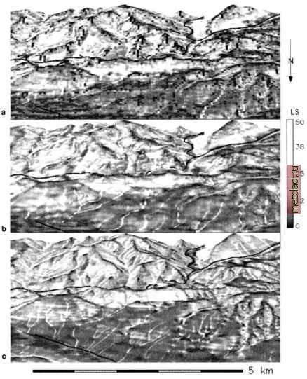

Figure 12.1. LS factor computed at a) 30 m resolution using the original Speafish integer DEM, b) 15 m resolution using the re-interpolated floating point DEM, c) 10 m resolution using the new USGS DEM from National Elevation Dataset. The center of this zoomed-in area is located at -103.68632, 44.42721 longitude, latitude. White areas have high topographic potential for erosion, dark grey areas are stable

When computing the LS factor, we multiply the flow accumulation by the resolution to get the upslope contributing area per contour width (it is in fact the flowline density multiplied by cell area in divided by cell width in m) and calculate the Equation 12.2 using r.mapcalc: