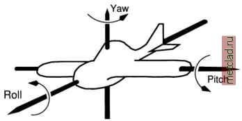Figure 10.5. Attitude angles of an aircraft

Since Omega and Phi could only be guessed from the aerial photos annotation bar (if present), approximate angles can be used. Only GPS-supported flights can provide these data accurately.

Then default values for the ortho-rectification calculations have to be entered, to provide initial values for the internal iterative computations. Appropriate value can be derived from the RMS-error. In our example, we set all X, Y and Z to 10m. The question Use these values at run time? (1=yes, 0=no) we use 1 :

Please provide the following information:

Initial Camera Exposure X-coordinate Meters:

Initial Camera Exposure Y-coordinate Meters:

Initial Camera Exposure Z-coordinate Meters:

Initial Camera Omega (roll) degrees:

Initial Camera Phi (pitch) degrees:

Initial Camera Kappa (yaw) degrees:

593933 4926053

12192

-90

Apriori standard deviation X-coordinate Meters: Apriori standard deviation Y-coordinate Meters: Apriori standard deviation Z-coordinate Meters: Apriori standard deviation Omega (roll) degrees: Apriori standard deviation Phi (pitch) degrees: Apriori standard deviation Kappa (yaw) degrees:

0.01 0.01 0.01

Use these values at run time? (l=yes, 0=no)

Now the oblique camera position and additional initial parameters are defined, and we return to the main menu and continue with the step 7. Compute ortho-rectification parameters and the subsequent procedure as described in the section above.

10.4. SEGMENTATION AND PATTERN RECOGNITION FOR AERIAL IMAGES

Aerial photos can be used for land use/land cover classifications similarly as the satellite data. However, because often only a single channel is available, either in black-and-white, in visible colors or in the infrared spectral range, the reclassification of aerial photos is different from satellite images. Image segmentation is a method for semi-automated feature extraction, such as the land use/land cover classes or edges from remote sensing data. A segmentation algorithm is implemented in the SMAP module i.smap which we already introduced in Section 9.8.3 for multi-channel satellite data.

The SMAP algorithm exploits the fact that nearby pixels in an image are likely to belong to the same class. The module segments the image at various scales (resolutions) and uses the course scale segmentations to guide the finer scale segmentations (image pyramid). In addition to reducing the number of misclassifications, the SMAP algorithm generally produces results with larger connected regions of a fixed class which may be useful in numerous applications. The amount of smoothing that is performed in the segmentation is dependent on the behavior of the data in the image. If the data suggest that the nearby pixels often change class, then the algorithm will adaptively reduce the amount of smoothing. This ensures that excessively large regions are not formed. The SMAP segmentation algorithm attempts to improve segmentation accuracy by segmenting the image into regions rather than segmenting each pixel separately.

The size of the submatrix used for segmenting the image has a principle function of controlling memory usage; however, it can also have a subtle effect on the quality of the segmentation in the SMAP mode. The smoothing parameters for the SMAP segmentation are estimated separately for each submatrix. Therefore, if the image has regions with qualitatively different behavior, (e.g., natural woodlands and man-made agricultural fields) it may be useful to use a submatrix small enough so that different smoothing parameters may be used for each distinctive region of the image.

Generating a training map. The module i.smap runs with single images as well as multispectral images. The raster polygons resulting from the segmentation process may be vectorized later with r.poly. To reclassify, i.smap requires a training map containing spectral signature. This training map contains numbered raster polygons which cover selected areas with homogeneous land use/land cover. The pixels inside a training area are considered to be spectrally similar. The training map is analyzed by i.gensigset which generates statistical information from the input aerial image based on the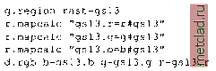

results in three pseudo-color channels which may be used for the segmentation. However, when working with 24bit images, the information contents is certainly higher.

Sometimes it is useful to generate and additionally use synthetic channels for the classification. For example, the module r.texture creates raster maps with textural features from image channels. The textural features are calculated from spatial dependence matrices at 0, 45, 90, and 135 degrees within a given moving window. For details, please refer to the related manual page.

A sample segmentation session. A sample segmentation procedure for the aerial image gs13 which was previously ortho-rectified into the Spearfish LOCATION may be performed as follows:

g.region rast=gsl3

i.group group=segment subgroup=segment in=gsl3

♦digitizing training areas such as fields, forest, roads etc, #save as map training : r. digit

d.rast training

♦generate class statistics from training map: i.gensigset training gr=segment sub=segment sig=smapsig

training map. The training map can be digitized (r.digit or v.digit with v.to.rast subsequently). The image statistics derived by i.gensigset is input to i.smap. As opposed to the Maximum Likelihood Classifier algorithm which operates pixel-wise, the SMAP also considers spectral similarities of adjacent pixels. The module i.smap expects the aerial image listed in an image group and subgroup.

If the aerial photo is a color image, it may be analyzed in three channels. During import, a 24 bit aerial color image can be split into the red, green and blue channels. Also black-and-white images can be roughly split into three pseudo-color images with r.mapcalc (# operator, see Section 5.2). The # operator can be used to either convert map category values to their grey scale equivalents or to extract red, green, or blue components of a raster map layer into separate raster map layers. The # operator has three forms: r#map, g#map and b#map. These extract the red, green, or blue pseudo-color components in the named raster map, respectively. For example,