
|
|
|
|
Главная --> Промиздат --> Map principle (the latter is not implemented in GRASS) can be found in McCauley and Engel, 1995. Summary of the standard reclassification techniques. As explained above, GRASS provides several options to reclassify multispectral data. Table 9.1 summarizes the available main reclassification techniques. 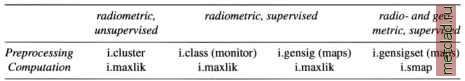 Table 9.1. Classification methods in GRASS NOTES 1 SAR User Guide from Alaska SAR Facility, http: www.asf.alaska.edu/SciSARuserGuide.pdf Remote Sensing Core Curriculum (RSCC), http: www.research.umbc.edu/~tbenjal/umbc7/ santabar/rscc.html ISPRS tutorial collection, http: www.isprs.org/links/tutorial.html 2 Imagery data set, http: grass.itc.it/data,html 3 GLCF Maryland LANDSAT Data for Spearfish (SD) region, ftp: ftp.glcf.umiacs.umd.edu/glcf/Landsat/WRS2/ p033/r029/ 4 NHAP documents, http: edc.usgs.gov/products/aerial/nhap.html 5 Xgobi/Ggobi software, http: www.ggobi.org 6 Atmosphere model 6S (Msix) software, http: www-loa.univ-lillel.fr/informatique/ system gb.html 7 Generating a surface temperature map from LANDSAT-TM7 channel 6, see Landsat 7 Science Data Users Handbook, http: landsat7.usgs.gov/resource.html 8 Asterweb (ASTER/TERRA), http: asterweb.jpl.nasa.gov Chapter 10 PROCESSING OF AERIAL PHOTOS Aerial photography provides a common base for large scale mapping. It has been widely used for creating and updating maps as well as for maintaining up to date GIS databases. Aerial photos can be used to extract georeferenced data representing topography, landforms, vegetation cover as well as man-made features. Besides creation of thematic maps, area and distance measurements at a large scale (in comparison to satellite-based methods) are often performed. Digital processing of aerial photos in GRASS allows the user to incorporate them into a GIS database. To minimize distortions, mainly displacement due to relief and airplane attitude, orthophotos are generated from (scanned) aerial photographs using a digital elevation model and a referenced map. They combine the characteristics of an aerial photo with the geometric qualities of a map, showing all objects in their precise geographic position. In the first part of this chapter we introduce generation of orthophotos, in the second part we explain image segmentation of aerial photos for land use classification and edge detection. 10.1. BRIEF INTRODUCTION TO AERIAL PHOTOGRAMMETRY Before going into details of generating a digital orthophoto, we describe the basic terminology used in aerial photogrammetry. Aerial photos are usually taken with overlap of around 60% for stereoscopic analysis; however, this method is not covered here. This chapter focus is on vertical aerial photos; however, a brief description of oblique aerial photos processing is included in Section 10.3.3. The aerial photo geometry is shown in Figure 10.1. Assuming that the aircraft which takes the photos moves (in the ideal case) over the target area without any deviation, the plumb line from the camera will be perpendicular to the horizontal ground plane. This case is called a true vertical image. The plumb line is also called the optical axis. Up to deviation of 3° in each direction, the image is called a tilted vertical image. If the inclination exceeds 3°, it is referred to as an oblique image. The nadir (also called plumb point) is the point on the earths surface (datum plane) which lies exactly below the recording camera. If a photo is taken without deviations from the plumb line, then the nadir will be in the image center (principal point). If the aircraft was tilted (oblique photo) then the principal point is not identical with the nadir. The principal point is found by connecting opposite fiducial 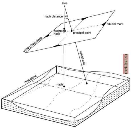 Figure 10.1. Aerial photo terminology (adapted from Neteler, 2000:178)
|