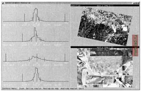Figure 9.17. Sample screen of interactive training area identification with i.class (SPOT-1 PAN image, Spearfish region)

After starting i.class., select an image group and subgroup. Then provide a name for the Result signature file . It will contain the spectral signatures for the later reclassification process. Next is the Seed signature file which allows us to read in signatures from a previous run (e.g. in case you interrupted this procedure). Skip it for the first run. Then specify a Cell map to be displayed which may be a previously generated natural or false color composite. This map, if not included in the image group, will not be considered for the image statistics. The monitor display becomes divided into three parts. In the upper right corner, you see the image. In the lower right corner, zoomed map portions will be displayed when using the ZOOM function. In the left section of the monitor, histograms for the selected training areas for all channels will be displayed. The training areas can be digitized by using the DEFINE REGION and the DRAW REGION buttons. When digitizing using the mouse, a vector line is drawn around the first training area. Keep in mind that the training area should cover a unique land use. To close the drawn polygon use COMPLETE REGION and leave the DRAW REGION menu with DONE . An example screen is shown in Figure 9.17. To verify the cluster statistics, click on ANALYZE REGION . Now the i.class module will search for spectral signatures based on the current training area within the image. The resulting histograms are shown in the left column of the monitor. The

next step is to determine the class assignment to the image - the spatial distribution of the current spectral signatures can be overlayed as filled polygons with DISPLAY MATCHES (you can select a color for the area). If desired, the standard deviation can be set to a different value ( SET STD DEVs ). This way, you can try to improve the cluster statistics and display the matches again. After displaying the matching areas, you are asked whether to accept this signature. If yes, you can specify a Signature description in the terminal window for this spectral signature. You can then continue to digitize the next training area. With some experience, you will become familiar with the concept of this module. Please note that the vector lines of the digitized training areas are not stored. See the next paragraph for an alternate approach based on retrieving training areas from auxiliary maps.

To obtain good results, you should not digitize border pixels of any land use patch because such pixels often contain mixed spectral signatures. It is also important not to digitize very small areas since these will be ignored for statistical reasons (i.class will print a warning message accordingly). Once you leave this module, the generated spectral signatures will be stored.

The spatial assignment of the data set pixels to the classes is done with i.maxlik. Specify the file generated by i.class as the Result signature map . The other settings are the same as described in the previous section. Finally, the reclassification map and the Reject threshold map are created.

Generating training areas from auxiliary maps. When additional maps with information about the current land use are available, they can be used to extract training areas. It is also useful to digitize training areas independently from i.class and store them in a separate map for later use/verification.

For raster maps, r.mapcalc (if-conditions) will be useful, for vector maps it will be the v.extract module. If training areas need to be digitized from a map, v.digit can be used (see Section 6.1.2). After digitizing, vector areas have to be converted with v.to.rast to a raster map. It is very important that the training areas are assigned a vector label, for example, within v.digit. Otherwise unlabeled areas will not be converted by v.to.rast. It is also possible to digitize from a raster image with r.digit.

The training map in the raster model is input for i.gensig. This module creates a signature file using the training area statistics similar to i.class. The spatial assignment of the pixels is subsequently handled by i.maxlik.

Partial supervised reclassification. The partial supervised reclassification is similar to the above-described unsupervised reclassification. The difference lies in the incorporation of training areas, which have to be defined prior to the application of i.cluster using i.class or i.gensig. After preparing spectral signatures from training areas, the clustering mod-

ule i.cluster is started and the Result signature file is generated with i.class or i.gensig is used as Seed signature for i.cluster. Finally the i .maxlik is used to generate the reclassification map and Reject threshold map . Beyond this step the procedure is the same as for the unsupervised classification.

Also, in the reverse order, the hierarchical classification is a way to derive thematic maps from satellite data. Based on an unsupervised reclassification, potential training areas are identified and stored in a map. This map is a basis for a supervised reclassification as shown above. As signature files can be used across the modules, better results are eventually achieved through an iterative approach rather than a straight-forward classification.

9.8.3 Supervised combined geometric and radiometric reclassification

GRASS provides an additional sophisticated supervised reclassification tool. The algorithm is a combined radiometric/geometric reclassification method which is called SMAP - sequential maximum a posteriori - estimation . Unlike the pixel-based approach described above, this method uses an image pyramid approach which also takes neighborhood similarities into account (Schowengerdt, 1997:107, see also Ripley, 1996:167-168). This combination leads to a significant improvement of the reclassification results (Red-slob, 1998). A second advantage is that the module also accepts a single channel data, so it can be used for image segmentation which we demonstrate later in Section 10.4. The SMAP implementation module is i.smap.

The steps for a SMAP-classification are as follows. First the data set images are joined into a group with i.group. Training areas have to be digitized with v.digit, r.digit or generated from existing vector or raster maps. The training areas map has to be a raster map. Note that the number of training areas defines the number of classes. Similarly to the other reclassification methods, the training areas should cover several pixels; otherwise they will be ignored if the pixel number is too small. The spectral signatures are generated from the training map with i.gensigset. This module first queries the name of the training map, then the group and subgroup names. The module creates a Subgroup signature file which corresponds to the above mentioned Result signature file .

From the spectral signatures, the supervised reclassification can be performed with i.smap. Again, group and subgroup have to be entered, followed by the name of the recently generated Subgroup signature file . After this, the computation will be started.

With a sufficient number of training areas, the results of this algorithm are superior to the MLC. A comparison of SMAP, MLC, and the ECHO reclassifier