When reclassifying multispectral satellite data, the image data set is analyzed pixel-wise, with the values of all channels being taken into account for each pixel. The number of pixels covering the same geographic region depends on the number of channels. This group of pixel values describing the same small area is called the spectral vector. It describes its specific position in the feature space (compare Figure 9.5 earlier in this chapter) which contains all spectral vectors. Within the feature space, the reclassification algorithm tries to separate similar spectral vectors which vary depending on the observed object types as soil, vegetation, water bodies etc. Similar spectral vectors will be assigned to the same class. All classes are finally stored in a thematic map where each class describes the dominating land use type.

A problem for the reclassification process are local variations which result from changes within and between the observed objects, slope and aspect changes of the terrain, and variations of the atmospheric conditions (haze, dust, clouds etc.). Depending on the observed area, data have to be radiometrically preprocessed as described in the previous section to minimize influences from slope/aspect and atmospheric effects.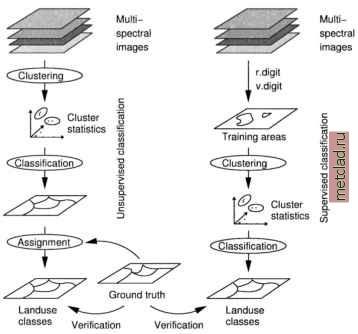

Figure 9.16. Unsupervised (left) and supervised (right) classification procedures for multispectral data

In general, two strategies are common for the reclassification of remote sensing data: unsupervised and supervised classification methods, which are outlined in Figure 9.16. For both methods, the reclassification process requires two major steps. The data have to be analyzed for similarities in their spectral responses and the pixels have to be assigned to classes. The unsupervised method is fully automated based on image statistics, but it delivers only abstract class numbers. The main task then is to find a reasonable number of clusters/classes and assign ground truth information to these classes. The supervised reclassification requires user interaction, as training areas covering known land use have to be digitized. Image statistics are automatically derived from these training areas and used for the final reclassification.

Common reclassification methods (MLC - Maximum Likelihood classifier as described in Sections 9.8.1 and 9.8.2) are pixel-based. GRASS additionally provides a different method (SMAP - Sequential Maximum A Posteriori classifier, see Section 9.8.3) which also takes into account that neighborhood pixels may be similar. The fact that a neighborhood of similar pixels will lead to spatial autocorrelation is used to improve the result. Altogether, four different approaches for satellite analysis within two main groups of reclassification methods are available:

Radiometric reclassification:

- Unsupervised reclassification (i.cluster, i.maxlik using the Maximum Likelihood reclassification (MLC) method), supervised reclassification and, combined,

- partial supervised reclassification (i.class, i.gensig, i.maxlik),

Combined radiometric/geometric supervised reclassification (i.gen-sigset, i.smap using the Sequential Maximum A Posteriori reclassifi-cation (SMAP) method)

A common problem in remote sensing of the environment are mixed pixels which cover various objects (field borders, urban areas, etc.). In this case, the mentioned methods will assign the pixel dominating object to a class, usually at a low confidence level. If appropriate, masking out settlements where lots of mixed pixels appear may be considered. Subpixel analysis methods such as Spectral Mixture Analysis are a way to overcome this problem (for a GRASS implementation see Neteler, 1999).

Other reclassifiers such as Artificial Neural Networks (ANN), k-Nearest Neighbor Classification (kNN), Support Vector Machines (SVM), and other methods are implemented in the R statistical language. They can be linked to GRASS using the GRASS/R interface; for an introduction to R, see Section 13.2.

9.8.1 Unsupervised radiometric reclassification

Unsupervised reclassification is the automated assignment of raster pixels to different spectral classes. The assignment is based only on the image statistics. The unsupervised classification is a two-step approach. First, a clustering algorithm groups pixel values with similar statistical properties according to user definitions of minimum cluster size, separability, number of clusters, etc. This approach is similar to the creation of a map legend, where the number of signatures existing in a map is identified and visualized. The pixel clusters are image categories that can be related to land cover types on the ground. The iterative clustering algorithm first computes the cluster mean values and covariance matrices (module i.cluster), adjusting these values while reading the image data set. The idea is to identify pixel clouds from the feature space which have similar reflectance values in the various channels. Each pixel cloud, grouped into clusters which represent land use classes, characterizes the spectral signature of a certain object which will be assigned to a class later on.

This cluster information is used to perform the spatial assignment of the individual pixels to the derived clusters (module i.maxlik). The MLC determines which spectral class each cell in the image belongs to with the highest probability. Internally, a Chi-square test is run with changing thresholds until a predefined convergence is reached (stability of the pixel assignment during the iteration steps). The result is a new map containing the classes. The MLC also stores the confidence level for each pixel belonging to a certain class in a second map. This map is called reject threshold map layer or rejection map and contains one calculated confidence level for each reclassified cell in the reclass map. High values in the rejection map represent a high rejection probability for the assigned class. One of the possible uses for this map layer is as a MASK, to identify cells in the reclassified image that have the lowest probability of being assigned to the correct class. It is important to know that MLC assumes that the spectral signatures for each class are normally distributed (i.e., Gaussian in nature) which is often unrealistic. For a detailed discussion, see various remote sensing books such as Mather, 1999.

First step: Clustering of image data. The unsupervised reclassification starts with collecting the image channels of interest (i.e. for optical data usually all reflective channels without thermal channel) into an image group using i.group. It is also important to generate a subgroup (menu item 5 in i.group) containing the same channels because the classification modules will ask for the subgroup name.

The clustering process is performed with i.cluster. A set of parameters has to be specified to control the clustering. It is important to set the initial number of classes used for the first iteration ( number of initial classes ); for other parameters, you may use default values for the first try. They have the