9.6.1 Matrix Iter: Spatial convolution Altering

Matrix filters can be used to locally modify the spatial frequency characteristics for an image. These modifications are based on calculations considering the neighboring raster pixels in a 2D spatial convolution process (for theoretical details, refer to Richards and Xiuping, 1999:114-116). These spatial convolution filters operate in spatial domain and are an alternative to frequency domain filters (such as Fourier Transformation). Spatial convolution filtering is well suited for:

high and low pass filtering (sharpening, blurring), averaging; edge detection by direction and gradient filters; morphological filters; preprocessing for image segmentation.

In the next part, we will describe high and low pass filtering and edge detection. In GRASS, two methods are available to define matrix filters. Either the module r.mapcalc or the module r.mfilter can be used.

The use of r.mapcalc is less convenient, as every matrix element has to be addressed with relative coordinates to the central cell. The format to address neighbor cells to the center is map[r,c], where r is the row offset and c is the column offset. For example, map[0,2] refers to the same row as the center cell and two columns to the right of the center cell, map[-2,-1] refers to the cell two rows up and one column to the left of the center cell. This syntax permits the development of neighborhood-type filters for one single map or across multiple maps. As a simple example, we define a 3x3 low pass filter. The filter equation for the each center cell

is coded as:

r . mapcalc lowpass= (map [1,-1] +map [1,0] +map [1,1] +map [0, -1 ] -t \ map[0,0]+map[0,1]+map[-1,-1]+map[-1,0]+map[-1, 1])/9.

You may try this example with the spot.ms.1 image. Further examples for r.mapcalc matrix operations are described in Shapiro and Westervelt, 1992.

A convenient way to perform spatial convolution filtering is to use r.mfilter with a matrix template defined in an ASCII file. We extend our first example to a 7x7 median filter which filters existing sharp contrasts in a raster map. This is effectively a low pass filter. The filter definition has to be stored in an ASCII file, for example, lowpass: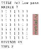

The mean value is preserved if the sum of the filter values equals the line-number * column-number. Every cell within the moving window is multiplied by 1. The results are summed up and finally divided by DIVISOR 49 (product of 7 * 7 * 1). To see how this works, the filter may be applied to the

SPOT-1 HRV1 channel:

r.mfilter spot.ms.l out=msl.lowpass filt=lowpass r.colors msl.lowpass col=grey.eq d.rast msl.lowpass

The color table may be set to grey or grey.eq with r.colors as in the example above.

Two types of filters are possible: sequential and parallel filters. Sequential filters (TYPE S) use the modified neighboring raster cell values for calculation of the central cell, while the parallel filters (TYPE P) use the neighboring cell values of the original map. Directional filters should be set up as parallel filters. Further information related to these types can be found in the manual page for r.mfilter.

Another example is a high pass filter for sharpening an image. It can be defined as follows (we store it in an ASCII file highpass):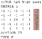

In this example the central cell of the window is weighted by 24, while the other cells have weight -1. The entire matrix is finally divided by 25 and its values are stored in a new map. Again, we apply it to the map spot.ms.1:

r.mfilter spot.ms.l out=msl.highpass filt=highpass r.colors msl.highpass col=grey,eq d.rast msl.highpass

The resulting map shows enhanced high frequencies (at the same spatial resolution). Note that a filter definition file may also contain multiple filters which will be applied to the image subsequently.

The only limitation of r.mfilter in comparison to r.mapcalc is that only integer numbers are accepted in a filter matrix. If you want to use floating point numbers or trigonometric functions, r.mapcalc must be used instead. The latter is also well suited for a thresholded binarization used to extract selected features (if-condition).

9.6.2 Edge detection

Edge detection is an important issue in remote sensing. An edge is defined as a significant change of the pixel values (DN) from one pixel to another. Related filters are also called gradient filters (Schowengerdt, 1997:246-247) such as Sobel, Robert, or other filters. The filter rules to define a Sobel edge detector for r.mfilter are shown in the next example. This filter sobel.filt is two-fold, as it can operate in north-south and east-west direction:

TITLE 3x3 Sobel (edge detection)

MATRIX 3

-I 0 I

-2 0 2

-10 1

DIVISOR 1

TYPE P

MATRIX 3 12 1 ООО -1 -2 -I DIVISOR 1 TYPE P

To apply it to the spot.ms. 1 image, we run:

r.mfilter in=spot.ms.l out=ms1.sobel filt=sobel.flit r.colors msl.sobel col=grey.eq d.rast msl.sobel

You can use r.mapcalc for a binarization (if-condition):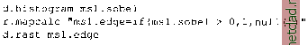

To achieve useful results, additional filtering is required before trying to extract edges. To skeletonize (thin) edges, you can use r.thin:

r.thin msl.edge out=ms1.edge.thin d.rast msl.edge.thin