where n is the number of required GCPs and p is the order of polynomial used for rectification with i.rectify. According to this formula, a third order polynomial transformation (p = 3) requires at least n=10 GCPs. It is recommended to always define more GCPs than the bare minimum. For example, for a third order polynomial transformation, at least 15 GCPs should be identified. Note that for image rectification second or third order polynomials are usually used. It is also important to use GCPs which are homogeneously distributed throughout the image.

The GCPs are stored in an ASCII file POINTS within the current LOCATION under a subdirectory group/<groupname>. Such a file is written automatically when r.in.gdal finds GCPs during the data import in the input data set. In this case, you can check the GCPs accuracy within i.points ( ANALYZE menu entry) which will load an existing POINTS file.

Rectification of the image data set. Based on GCPs stored in the POINTS file, the module i.rectify performs the image rectification into the target LOCATION. Unlike projection and transformation between coordinate systems using r.proj, which is based on mathematically defined projection

the terminal window. Using several maps to get the GCPs is recommended; in our example the fields map or others can also be used. It is easy to change the displayed channel or reference map during the GCP collection. Figure 9.6 shows a typical screen for geocoding a satellite image in GRASS with i.pointsB.

The ANALYZE menu allows us to check the geometrical accuracy of the GCPs. A misplaced point can be disabled (and also enabled again) by double clicking a row in the points table. A disabled point pair is shown in the image and in the list in red. At the bottom of the table, the RMS error (root mean square error) is shown; you should try to reach accuracy of half pixel size. For the SPOT-1 example this means the maximum 10 m RMS error when geocoding a multispectral channel with 20 m pixel size. The GCPs are used for all images in the image group; in our example, for the three multispectral channels. When working with i.vpoints and referencing against the roads vector map, it might be easier to achieve high accuracy.

The number of required GCPs depends on the rectification method. For a linear transformation 4 points are sufficient, preferably selected in the corners of the image. Non-linear polynomial transformations from 2nd to pth order require more points. The minimum number of points can be calculated as follows:

models, i.rectify uses linear or higher order polynomials to warp a source image to a target LOCATION.

After startup of i.rectify, the image group has to be specified. For our example we select again the group spotmss. The module then asks for the order of polynomials to be used for the transformation ( order of transformation ). The following transformation methods are usually used:

1 Helmert (similarity) = linear: stretching and rotation (needs 4 GCPs);

2 bilinear (affine): allows for stretching and rotation at different scales, able to correct image intrinsic earth curvature (needs 6 GCPs or more);

3 cubic: allows also for earth curvature correction, may tend to overcorrec-tion (needs 10 GCPs or more).

After the order selection, proceed to the next screen with <ESC><ENTER>. Specify new file names for the images that will be stored in the target LOCATION. You may choose the same names or different ones, use list to check which names are already in use. After leaving this screen, the module asks for two options:

Please select one of the following options

1. Use the current region in the target location

2. Determine the smallest region which covers the image

>

Both options are used to define the extent of the images in the target LOCATION. The first will clip the image to the current settings and also use the GRID RESOLUTION currently defined in the target LOCATION. Before running i.rectify, setting the resolution in the target LOCATION to the image resolution is recommended. For verification or adjustment, you may temporarily restart GRASS with the Spearfish LOCATION and come back to the Imagery LOCATION to continue (for this interrupt i.rectify and restart it later). There is, however, an alternative to that: The second option in the above menu allows the user to modify all parameters in a new screen which is similar to the LOCATION definition screen. The default settings are the maximum region extent and resolution from the target boundary coordinates and the image size. You may adjust the values as desired.

After selecting option 1 or leaving this screen when using option 2 (here you are finally asked whether to set the target LOCATION to the new values), i.rectify starts to rectify the image(s) in background. This may take a while, depending on the data size and computer speed. The module sends an email when it is finished. After completion of the calculations, the geocoded satellite data are integrated into GIS and may be analyzed along with other GIS data in the target LOCATION. The panchromatic channel spot.p needs to be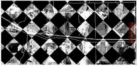

Figure 9.7. Pattern-overlay to verify the geocoding accuracy of a satellite image to a raster reference map

rectified into Spearfish LOCATION using the same procedure as we have just described.

Checking the accuracy. To evaluate the quality of the geocoding process, potential spatial shifts between the rectified channels and the reference map(s) should be verified. The rectified channels can be either displayed in different GRASS monitors or, better, overlayed in small patterns. A pattern oriented overlay method of different data sets can easily be done with MASKs and r.mapcalc. We use a rotated square pattern which alternately shows a channel and the reference map within the squares. To generate this pattern, bi-narized thresholded sine curves are used to generate the MASKs. We display the roads map and the geocoded SPOT-1 PAN channel as follows:

g.region -p rast=spot.p #remove MASK if present: g.remove MASK

v.to.rast roads out=roadslOm ♦generate binary square pattern mask: r.mapcalc MASK=if ( (sin(5*row()) + sin(5*coli

d.rast spot.p g.remove MASK

♦generate inverted binary square pattern mask; r.mapcalc MASK=if( (sin(5*row()) + sin{5*col<

d.rast -o roadslOm g.remove MASK

) ) ) > null (

) ) ) > 1, nul

0.0,\ ) , 1)

0.0, \ 10)