set can be directly imported into the target LOCATION and used for further analysis. If it is in a different coordinate system, the data set must be imported into its own LOCATION and projected to the target LOCATION with r.proj (see Section 3.3.2). It is important to check the geometrical accuracy with reference maps.

Case 2: the image data set is not geocoded, but GCPs are present.

When importing the data with r.in.gdal, existing GCPs are extracted into a GRASS POINTS file (used later by i.rectify). If the GCPs represent the four corner points, a Helmert (similarity) transformation can be performed to transform the data into a georeferenced LOCATION (first order polynomial transformation). However, as this linear transformation only stretches and rotates the image, it is not very accurate for satellite images which may also contain distortions within the image. Improvements can be achieved by adding more GCPs and using a higher order polynomial rectification method. As mentioned in the import section of this chapter, the extracted GCPs coordinates, which are usually provided as latitude-longitude coordinates, can optionally be projected on the fly to a target coordinate system. This will be explained in greater detail later.

Case 3: the image data set is not geocoded, no GCPs are present. First, GCPs within the image and on a reference map have to be identified. GPS data can be used instead of the points on the map. The geocoding process in GRASS then requires three steps. Create a source LOCATION which contains the satellite data set. Then create a target LOCATION (usually projected) into which the raw data set will be rectified. This target LOCATION contains reference map(s) for GCPs identification. Finally, after a sufficient number of spatially accurate GCPs is identified, the rectification of the input image or image group from the source to the target LOCATION is performed.

Ground control point identification. GRASS provides tools for on-screen identification of ground control points on digital maps and for assigning points from GPS measurements. Four types of image rectification are generally possible: image to image (staying in xy-coordinates), image to raster map (georef-erencing to raster map), image to vector map (georeferencing to vector map), and image to keyboard specified coordinates (referencing against known points such as GPS data). As mentioned above, when working with multi- or hyper-spectral data, all channels of interest should be assembled into an image group with i.group. As an example, we geocode the SPOT-1 HRV data as provided in the LOCATION imagery. First, we select the SPOT-1 HRV data in a group (the PAN image is shifted within the LOCATION imagery and has to be rectified in an extra procedure):

LOCATION: imagery

GROUP: spotmss

MAPSET: markus

Please mark a x by the files to be added in group [spotmss] MAPSET: PERMANENT

gsl3.1 spot.p

gsl4 .1

nhap.1

nhap.2

nhap.3

nhap.enh

spot.comp

x spot.ms.1 x spot.ms.2 x spot.ms.3

You can select a channel by writing an x; delete a selection by overwriting the X character with blank. Leave the selection screen with <ESC><ENTER> and confirm the selection. In the main menu, you can optionally specify a subgroup, which is required for some GRASS image processing tools. For our example, we can leave i.group with <ENTER>. Note that you can also use the module on the command line.

Before starting the GCPs identification, the target LOCATION (in our case the spearfish) has to be specified with i.target:

i.target group=spotmss location=spearfish mapset=userl

For the graphical identification of ground control points, GRASS provides a few modules: i.points to reference to a raster map, i.vpoints to reference to a vector map, and i.pointsB (under development), which combines previous modules and i.ortho.photo. Also, ortho-image generation from satellite images will be possible when using i.pointsB with i.rectifyB by incorporating the elevation and a geometrical sensor model.

For our SPOT-1 example, we use the module i.points to interactively define GCPs in the GRASS monitor. The GRASS monitor must be open and the

The following screen appears; enter the image group name spotmss:

LOCATION: imagery i.group MAPSET: markus

This program edits imagery groups. You may add data layers to, or remove data layers from an imagery group. You may also create new groups

Please enter the group to be created/modified

GROUP: spotmss (list will show available groups)

Leave the screen with <ESC><ENTER> and accept it with y. Now you reach a new screen where you can select the images: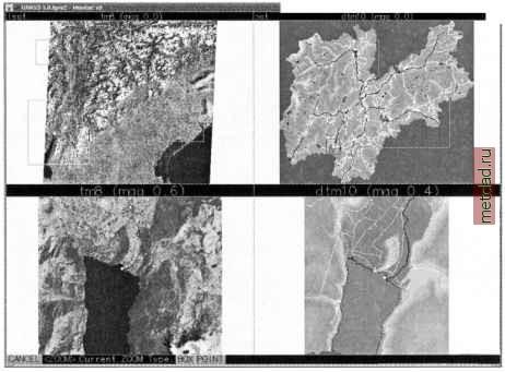

Figure 9.6. Geocoding of a satellite image to raster/vector reference maps with i.points3

i.points started. It queries for the image group; here, specify the recently created group spotmss. An image from the image group can now be selected for display in the upper left half of the GRASS monitor. Select a channel from the list to plot it. This may also be an additional color composite included in the image group. Using the PLOT RASTER menu and clicking into the right half of the monitor, a reference map from the target LOCATION can be displayed (for our example, choose the raster map roads). Ground control points can now be assigned. It is important to use the ZOOM function in both maps to achieve high accuracy. A GCP is set by clicking with mouse at a point, first in the source image, then at the related tie point in the target map. The selection needs to be confirmed and an accepted point pair is drawn in green color.

For the first GCPs pair, you may start and zoom into a road intersection, both in the satellite image and the roads map (select ZOOM , then BOX , draw a box with the mouse). The zoomed image/map portions are shown in the lower half of the GRASS monitor (compare Figure 9.6). Remember from vector digitizing that useful points are located in the middle of road intersections, field corners, etc. Alternatively, the input method can be changed to KEYBOARD in the menu to directly specify coordinates for a point in the source map in

wtmmmmmi..........MMiiiirt