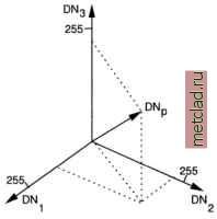Figure 9.4. Pixel in a three-dimensional feature space with digital number (adapted from

Schowengerdt, 1997:119)

areas are bluish. A geocoded SPOT-1 false color image is already included in the Spearfish LOCATION (spot.image).

We provide a more detailed explanation of color models and image composites in Section 9.7.

9.3.2 The feature space and image groups

The processing of data from a multispectral satellite sensor is based on the concept of feature space defined by the sensor channels. Together with the definition of an image group as a combination of multiple channels, this concept is a foundation for image classifications.

The feature space. The channels of a multispectral satellite sensor are considered to span a multi-dimensional coordinate system called feature space. For example, the three channels covering visible light (blue, green, red) span a three-dimensional coordinate system. Within the coordinate system (or feature space), every pixel reaches a certain position depending on the brightness levels in each channel. This position can be considered a vector in the multidimensional coordinate system. The brightness levels of the pixels in the different channels are called digital numbers (DN). Figure 9.4 shows the position of a pixel in a three-dimensional feature space, which may represent the blue (DNi), green (DN2), and red (DN3) specttum range.

The concept of feature space plays an important role in image classifications that are used to derive land use maps from satellite data. Classification methods are based on the idea that pixels containing the same land use are close to each other within the multi-dimensional feature space. The number of dimensions depends on the number of input channels. For example, a number of multispectral pixels which cover a forest will show similar spectral signatures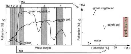

Figure 9.5. Left: Spectrum showing typical spectral response of common objects with LANDSAT-TM5 channels 3 (red) and 4 (NIR); right: Two-dimensional feature space of channels tm3 and tm4 with pixel brightness levels. Three pixels for each observed object (water, sandy soil and green vegetation) are shown with their brightness levels in 3 and 4. The feature space scatterplot (right) represents reflection per channel as appear in channels tm3 and tm4 (adapted from Neteler, 2000:158)

and therefore should be assigned to land use class forest . In the process of reclassification, many methods (e.g. cluster algorithm) group adjacent pixels in the multi-dimensional feature space and assign them to the same class. Figure 9.5 shows the relationship between the spectrum and a two-dimensional feature space spanned by the red and the near-infrared channel of LANDSAT-TM5. More details on image reclassification will be explained below.

For illustration, we display the feature space of two channels of the SPOT-1 satellite scene in the GRASS monitor (red and near-infrared channels):

g.region rast=spot.ms.2 dcorrelate . sh spot.ins.2 spot.ms.3

The pixel clouds from the red and near-infrared channels span the two-dimensional feature space, which will be partitioned in a reclassification to extract land use classes. However, in the above scatterplot, it is difficult to visually distinguish clustered areas. If you zoom into a small subregion of a SPOT-1 HRV channel and re-run the dcorrelate.sh script, the scatter-plot will be different, with easier to distinguish pixel clusters. For higher level graphical data analysis external software like R (compare Section 13.2) or XGobi 5 are recommended.

Image groups in GRASS. Since we are dealing with multi-spectral data sets, we need a method to bundle the channels which belong together. This helps when operating on multiple channels with identical geolocation. GRASS

9.4. GEOMETRIC AND RADIOMETRIC PREPROCESSING

In this section, we explain how to preprocess satellite data for further analysis. After geocoding the data set, we continue with radiometric preprocessing to statistically explore the data and to extract further information. To illustrate the applications, we again use the SPOT scene as well as the free LANDSAT-TM7 scene.

9.4.1 Geometric preprocessing

If the imagery data are analyzed in conjunction with other GIS data, geometric preprocessing is crucial. While it may be acceptable to use the image coordinate system for image-only analysis, for a combined image/map analysis and distribution of the results to other GIS users, a high quality geocoding is essential.

Geocoding is related to the terms ground control points (GCPs, also called tie points ) and projection . Ground control points are sites of known position within an image. They are used to perform an image rectification to a reference. These GCPs can either be the four corner points of an image or, preferably, distributed over the image. If available, GPS (Global Positioning System) data can be used as reference points.

General methods of geocoding. Depending on the data provider and the product level, the data set may already contain GCPs or it may be already geocoded. In the latter case, no further geocoding is needed, only potential transformation to the target coordinate system. The following situations can occur when obtaining a satellite data set:

1 the image data set has been already geocoded and projected by the data supplier;

2 the image data set is not geocoded, but contains the four corner GCPs;

3 the image data set is not geocoded, and does not contain any GCPs.

Case 1: the image data set is already geocoded. In this case, you have to verify whether the data are in the target coordinate system. If so, the data

offers a tool to group images by selecting the channels: i.group. Several multi-spectral image processing modules expect an image group, a few of them even need a subgroup (which may contain the same channels or a subset). Even when working only with a single image, this channel has to be assigned to a group. We are now ready to explore more complex remote sensing issues.