204 60

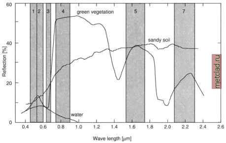Figure 9.2. Idealized reflection curves of green vegetation, sandy soil and water. For illustration the LANDSAT-TM5 channel filter functions except the thermal channel 6 are shown in background (curves as defined in 6S source code, Vermote et al., 1997)

Details on technical aspects of satellite sensors and their characteristics can be found in Kramer, 1996, Schowengerdt, 1997, and various other remote sensing textbooks.

Besides the different sensor types, satellite systems are also distinguished by their orbit: there are polar orbiting and geostationary satellite systems. The geostationary orbit is far from the earth (usually at 36,000 km above the earths surface) which allows the satellite a static position of the sensor in relation to the observed area. This orbit is used for weather and telecommunication satellites as they need to always watch the same area. Unlike that, near-polar orbiting satellites are rotating around the globe near the poles, covering the entire surface within a fixed range of days due to their own and the earths rotation. The orbits are near-polar oriented to enable the satellites to cross the earths surface everywhere at the same time. This leads to a constant solar illumination which is important for multitemporal analysis. Within this chapter we focus on methods for polar orbiting systems.

Resolution. An important aspect of satellite data is the image resolution. In particular, we have to distinguish between:

spatial (geometric) resolution;

spectral resolution;

radiometric resolution.

Spatial or geometric resolution is the spatial extent of each pixel as known from the raster data. For environmental satellite data, this resolution typically ranges from 1 m to 30 m. The sensor-specific geometrical resolution limits the usability of satellite images to certain map scales: Satellites such as the U.S. LANDSAT-TM7, the French SPOT HRV, and the Indian IRS-1D, with a pixel size in their multispectral channels ranging from around 20 m to 30 m, may be used for mapping at a scale of 1:75,000 to 1:250,000. Recently, high spatial resolution satellites with 1 m pixel resolution became operational, however, they provide only a few image channels which limits the number of classes for land use classifications.

Spatial resolution is closely related to geocoding. The satellite image is often distorted and registered in a non-georeferenced coordinate system. Based on ground control points (GCPs), the satellite image can be registered to a reference map. This process is called geocoding and is covered later in this chapter. If the satellite image is already geocoded, it can be imported directly into a georeferenced LOCATION.

The spectral resolution refers to the bandwidth of each channel. The bandwidth is the range of the spectrum measured by one channel. Figure 9.2 shows the bandwidths of LANDSAT-TM5 channels with respect to the spectrum and object spectra. Both the higher number of channels and the bandwidth of each channel improve the potential to distinguish objects in an image. For example, when studying crop conditions, phenology-driven signal variations are found in a narrow spectral range between the red and the near-infrared spectrum. Only when this range is covered by two or more narrow bandwidth channels can the effects be studied. Later on we will show how to merge channels with high spatial resolution and with those with high radiometrical resolution to improve classifications.

The radiometric resolution describes the signal dynamics within one image. While the LANDSAT-TM5 channels are effectively measured at 7 bit, other satellites have a radiometric resolution up to 12 bit (e.g. ASTER/TERRAs TIR channels) or even more. For technical details on the various satellite sensors, see the remote sensing textbooks, Kramer, 1996, or Web sites of the space agencies.

In general, a pixel in remote sensing has three parameters: space, wavelength and time (Schowengerdt, 1997:16). Based on these parameters, it is possible to derive thematic maps from satellite data using various methods for image classification.

9.2. SATELLITE DATA IMPORT AND EXPORT

Satellite data are provided in a variety of data formats and sometimes the user can choose according to her/his needs. Common formats are CEOS (unfortunately existing in various subformats), BIL, BSQ, GeoTIFF and others. In general two main format types have to be distinguished:

formats which contain one channel per file (SUN-raster format, TIFF and PNG format);

formats which contain one or more channels per file (BIL or BSQ format, CEOS (with various subformats), ERDAS/LAN, NCSA/HDF or HDF-EOS format).

Before working with satellite data in GRASS, you have to verify whether your satellite data are already geocoded because the import method depends on it. This information should be delivered with the metadata belonging to the data set. If there are no metadata present, there might be the chance to retrieve metadata from the image itself using the command gdalinfo (which is part of the GDAL library). When specifying the name of the image file as a parameter, gdalinfo prints metadata such as projection and boundary coordinates if the image format supports metadata storage.

After a general description of how to build the xy LOCATION, we will start to use the imagery sample data set provided for the Spearfish region. It is available at the GRASS Web site.2 Beside a SPOT-1 HRV/PAN scene, aerial photos such as NHAP (National High Altitude Photography) multispectral aerial photos and a black-and-white stereo pair with camera information are also included.

9.2.1 Import of raw and geocoded satellite data

Before importing the satellite data, a LOCATION has to be defined. This can be done manually through the GRASS interface or generated automatically with r.in.gdal.

Manual definition of a raw data xy LOCATION. Non-georeferenced, (raw) satellite data have to be imported into an xy LOCATION. This procedure is described in Section 3.2. The satellite data set can be imported us-

GRASS provides numerous modules devoted to image processing. Image data are processed using the raster data model; therefore, all raster modules can be applied. To distinguish the specialized image processing tools from the others, they are prefixed with i. (example: i.class).