Displaying sites. To change the symbol used for the site data, go to Panel Sites and open the site panel (Figure 8.3). It is similar to the vector panel - you can use it to add or delete a sites map layer, select the surface on which the current site data should be draped, and select the symbol, including its color and size. If you have 3D site data, you can also display them in the 3D position rather than draped over the surface. This is particularly useful when evaluating interpolation and smoothing of surfaces as you can see how much the surface deviates from the given data and where the highest deviations are.

Controlling light. Interactive light manipulation is useful for detecting noise or small errors in surfaces as well as for enhancing the 3D perception of surface topography and creating special effects. The panel Panel ~> Lights is used to change the lighting parameters such as the light color, brightness, ambient (dispersed) light and a position of light source (height and direction) by using the appropriate sliders and a square with puck. Interactive adjustment of lighting is made easier by a sphere which appears in the center of the graphics window and shows the current lighting effects as the changes are made (Figure 8.5). The sphere disappears when the surface is rendered, for example with

the Draw button.

Adding legend and labels. To add a legend, title, or other text to the images displayed by nviz, open the Panel Label panel that allows you to type in short text and place it in the graphical window with the mouse. The legend has options similar to the command d.legend and you can again place it with the mouse. The legend is then automatically redrawn with the image, to remove the legend, draw the surface with the button On switched off.

Displaying vector data. If you would like to choose a different color for your vector map or add an additional vector map layer, open the vector panel by choosing Panel Vectors (Figure 8.3). You can load the new vector map using the new button. After loading, the switch Display on surface(s) will be automatically activated for all surfaces (when working with multiple surfaces switch off those on which you do not want to drape your new vector data). You can adjust the line width and color by using the appropriate buttons. For example, select black for roads and then click on the name of the current vector file, select streams from the menu of available layers and change its color to blue. You can use Draw current in the vector panel to drape only the selected vector file. To render the surface with all vectors and sites draped over it, use the Draw button on the top of the movement panel. If the lines are not fully rendered, move them slightly above the surface using the Vect.Z slider.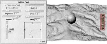

Figure 8.5. Interactive control of light aided by a sphere

Saving images, state and view settings. To save the created image, go to File - Image dump and select one of the formats that you want to use (SGI/RGB-Format, TIFF, PPM). You can transform the saved image to JPEG, Postscript or other formats using a graphics program such as gimp. To render and save image at high resolution (for example, at 5000 x 5000 pixels), use the full resolution PPM option. The image will be split, rendered piece by piece and then patched together.

Using File Save state you can save the settings of your current 3D visualization. You can restore the settings by File Load state . Using this capability, you can save and quit your work and then start it again without losing just the right light and view that you have found. It is highly recommended to save the state regularly so that you can go back and restore your settings at later time. You can also save your 3D settings in a GRASS 3d.view file using the Save 3d settings option from the File menu or load the settings from a previously created file to get specific viewing parameters.

8.2.2 Querying and analyzing data in nviz

To use nviz for both qualitative and quantitative analysis you can perform 3D queries. Choose Panel Whats Here? and activate the Whats here? switch. You can select which attributes you want to be included in the query using the button Attributes . In Figure 8.6 we query the active upper elevation surface with slope map draped over it. By pointing the mouse at a location of interest, get its coordinates including the elevation, the slope value, and a distance from previous queried location. You can also use nviz to perform small digitizing tasks in 3D by using Whats here? and piping the result into a file. The file can then be converted into a site file or a raster

file using nvizimport script. The principles used in the algorithm for 3D spatial query are described by Brown et al., 1995. If you have nviz compiled with Postgres support, you can directly query connected tables in PostgreSQL DBMS for vector and point data attributes.

Working with multiple surfaces. Multiple surfaces are by default displayed based on their 3D coordinates; however, their relative position can be changed using the position menu, which opens after clicking on the Panel Surfaces Position button. You can change the relative vertical position of a current surface using the z slider or you can move the surface around using the cross in a horizontal position square. Using this interface, you can arrange your surfaces within your graphical window in a way useful for visual analysis; for example, next to each other, as shown in Figure 8.7.

When comparing multiple surfaces, cutting planes can be very useful. Choose Cutting plane from Panel menu, select a cutting plane (you can have up to 8) and set its appropriate orientation using the Rotate slider. You can also slide the rotate slider to interactively cut through your surfaces, or you can slide the cross to move the cutting plane through the surfaces in fixed direction. The color of the cutting plane can be set to the color of the top (T) or the bottom (B) surface, blend (BL) of those two colors, grey (GR) or invisible (N) by switching on the appropriate button.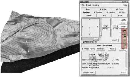

Figure 8.6. Interactive 3D query of elevation surface with slope map draped as color