
|
|
|
|
Главная --> Промиздат --> Map principle and use the interface to load your data. Alternatively, you can define the map layers that you want to visualize on the command line; for example, to view the DEM with streams, roads, and some site data from our Spearfish data set, run: nviz elevation.dem vect=streams,roads sites=archsites,bugsites The program opens a graphics window with a coarse model of the elevation surface and a control panel window. If you click on the DRAW button, the elevation model with the vector and site data draped over it will be shown at higher resolution. Depending on the size of your raster map, the surface may not be rendered at its full resolution and the view may not be optimal. In the following paragraphs, we explain how to adjust it to create a desired 3D view of studied area. Controlling the view. The position of the viewing point, viewing direction, perspective (zoom-in, zoom-out) and tilt of the surface can be adjusted using the Controls menu (Figure 8.3). Use the left mouse button to move the puck around the viewing direction square to change the position of viewer and the direction of view - the coarse model of your DEM will move simultaneously making it easier to find the desired viewing position. The perspective slider allows you to zoom-in and zoom-out while the height slider controls the viewing height. The zexag slider is used to interactively modify the z-exaggeration (it effectively multiplies the elevation data); note that it also changes the height of the view so you may need to re-adjust it. If you cannot achieve the desired view with the sliders or if you want to define an exact value for any of the viewing variables, you can type them into the related field and type <ENTER> to continue. To focus on an area off the center of your map, use the look here button to select a new center of view with a mouse click (pin your surface in your focus area). All movement of the surface will be centered around this point. To get an ortho view, click on the top button and use RESET button to get back to the default behavior. The twist slider allows you to tilt the displayed surface to simulate the view from a turning airplane. The surface with all other map layers will be rendered after each change. If you are using multiple steps to adjust the view of your surface, you can switch off this automatic rendering using the buttons in the upper part of the control menu. Modifying properties of surfaces. The viewed surfaces are managed using the options provided by the Panel Surfaces menu (Figure 8.4). In the upper part of this menu you can adjust the drawing style as well as the level of detail for the rendered surface. By default, the surface is rendered as colored polygons with Gouraud (smoothed) shading, using a coarser resolution while the surface is interactively manipulated. To change the surface display to a 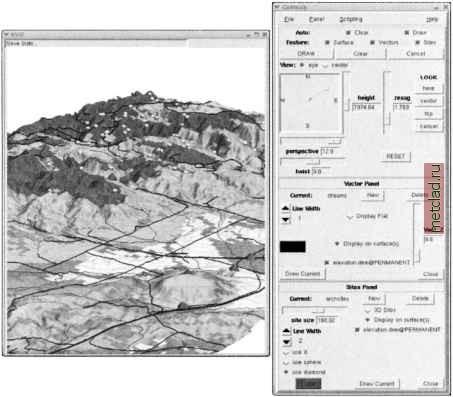 Figure 8.3. Spearfish geology map draped over a DEM with overlayed streams and roads as vector data, and archaeological and insect collection sites as point symbols (pyramids and spheres respectively) mesh (wire) or colored surface with a mesh, select the desired option from the menu under Surface style . For fast interactive manipulation, you can select wire from the Grid style menu. To render the surface at the current region resolution (as given by g.region), set the Polygon Resolution to 1 . Note that if the current resolution is higher than the resolution of the raster file used for topography, the raster file is automatically resampled leading to the discontinuous surface shown by Figure 5.3 (see Chapter 5). To speed up the rendering while exploring the viewing parameters you can lower the rendering resolution (increase the cell size) by choosing a higher value of polygon resolution. If you are using any style that involves wire, you can adjust its grid spacing with Grid Resolution . To drape a new color map over the surface select a new raster map using the color option from the Surface Attribute menu, for example soils.ph in 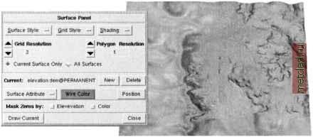 Figure 8.4. Displaying topography at multiple resolutions controlled in the upper part of the Surface menu, using multiple, masked-out surfaces our Spearfish example. After loading the raster map, use DRAW to render your elevation surface with the new color map (Figure 8.3). To overlay an additional raster map, you can use transparency. However, for its meaningful application, the raster map for transparency should be fairly simple. A possible use may be to suppress (lighten) the areas outside a studied watershed. To render only a subset of the surface, you can define a raster map to be applied as a mask using the mask option from the Surface Attribute menu. Masking can also be used to create a 3D view of topography with spatially variable resolution using nested grids approach (Figure 8.4). For example, assume that you have a 100 m resolution DEM for entire region and a 20 m resolution DEM for a smaller subarea. To create a multiresolution surface, set the resolution to 20 m by g.region and start nviz -q. Switch off all automated redraw buttons in the top panel and load the two DEMs using the Panel - Surface New button. Then, with the current surface set to the 100 m resolution DEM, define its mask using the 20 m DEM through the mask option from the Surface Attribute menu. Set Polygon Resolution to 5 (5 x 20 = 100) and render the 100 m resolution DEM using the Draw current button. You will get the surface with a hole in the area where the high resolution DEM is located. Then, select the 20 m DEM as current, set Polygon Resolution to 1 and render the 20 m resolution DEM with the Draw current button and save the image if it looks good. Depending on resolution, there may be a masked strip between the two surfaces, you can use a slightly smaller raster than the inserted DEM as a mask to ensure sufficient overlap.
|