from the true monitor pixel size. Before displaying maps in a frame, select it with the mouse as described above. An example with three frames in a GRASS monitor is shown in Figure 8.1.

As with any other window, you can adjust the GRASS monitor size using the mouse. To change its default size, use the UNIX environment variables GRASS HEIGHT and GRASS WIDTH either in /etc/profile or locally in $HOME/.grassrc5. If you are using tcltkgrass you can set the size in the CONFIG OPTIONS DISPLAY DIMENSIONS menu. These changes will become valid for your next start of a GRASS monitor. In order to save this new configuration for future sessions, you have to answer YES to SAVE CONFIG when leaving tcltkgrass.

You can add legend, scale, and text to your displayed map using d. legend, d.barscale, and d.text respectively. If you want to include this map in a presentation or a report, you can use a graphical program such as gimp to snapshot the window. Later, in Section 8.1.3, we show how to generate high resolution output as an image file with the PNG driver. You can display the legend in a separate monitor, frame, or you can just stretch your current monitor to make space for the legend and place it with a mouse using the -m option. For d. legend, you can use continuous colors for the continuous field data with the flag -s and discrete colors for raster map layers with categories (see examples in Chapter 12). For floating point raster maps representing continuous fields, it is appropriate to use the legend command with the -s option, creating a legend with smoothly changing colors, because in such maps the colors for each cell value are interpolated based on the values and colors given in the color table.

There is no legend tool yet for vector and site data - you need to use external graphical software to add it to the snapshot image. You can display labels for your raster, vector, or sites map layer by using d.rast.labels, d.vect.labels, and d.site.labels.

For raster data, working with color provides a powerful tool for extracting important spatial information and communicating it effectively. As we have explained in Section 5.1.1, the raster color table can be defined by r. colors. Besides selection from a set of predefined color tables you can define the colors by their names using the option color=rules, or you can copy a color table from another raster map using the option raster=mymap (see examples in Section 5.1.1). For a refined definition of colors you can use the red, green, blue (RGB) color description (see Section 9.7.1). To find suitable RGB values for a desired color, use any graphics tool provided by your system. For example, in gimp, find a palette under File ~> Dialogs ~ Palette . Select a palette suitable for your map and then click on the individual colors to get the RGB values which you can then use in r. colors. Besides the applications throughout this book, you can find examples of rules for creating the color ta-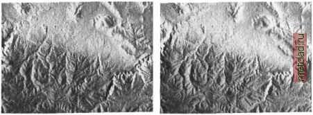

Figure 8.2. Shaded elevation maps: shade map with sun azimuth=270° from north (left) and shade map with sun azimuth=90° (right), sun altitude=30° above horizon (Spearfish data set)

bles in the Chapter 12, in the Section 5.4.4 and, of course, in the manual page for r.colors.

8.1.2 Creating a 2D shaded elevation map

To enhance the perception of topography represented by a DEM, a shaded elevation map can be generated quite easily. A special color transformation is used to prepare a translucent view of the DEM (or any other raster map) and the shade map. It is based on the IHS color transformation which is explained in greater detail in Section 9.7.1. First, we generate a shade map based on the sun position using the script shade. rel. sh. The name of the resulting shade map is created automatically by adding . shade name extension to the name of the elevation file. This map is then used to display the elevation.dem map layer with shaded topography by d.his:

shade.rel.sh altitude=30 aziinuth=270 elevation=elevation.dem d.rast elevation.dem.shade

d.his h=elevation.dem i=elevation.dem.shade

You may experiment with different values for altitude and azimuth when creating the shade map to highlight various topographic features. Figure 8.2 shows the effects for different sun azimuth angles. You can also apply shading to other types of surfaces when studying their structure.

If you want to save the shaded map into a file, use r .his instead of d. his. It creates three map layers representing the red, green and blue channels (because the original map is 24bit, it writes three 8bit maps). In our next example, we call themel.b, el.g, el.r. You can then use the module r.composite to combine the three color maps within GRASS into a single shaded elevation map dem.shaded:

r.his h=elevation.dem i=elevation.dem.shade b=el.b g=el.g r=el.r r.composite b=el.b g=el.g r=el.r out=dem.shaded d.rast dem.shaded

The module r.composite provides optional parameters to control the color levels to be used for each color component (default color levels per channel: 32). This default number of levels results into a total of 32768 possible colors (equivalent to 15 bit per pixel). Due to limitations in the GRASS display color model both r.composite and d.rast will significantly slow down if more colors are used. However, for human eye, this number of grey shades is quite sufficient. You can also export the three map layers and compose them into 24 bit shaded elevation image using external graphics tools. Alternatively you can export the map using r.out.ppmB which writes a 24 bit PPM file. Note that the composite shaded elevation map is only usable for visualization purposes as the elevation cell values are modified due to the shading.

8.1.3 Monitor output to PNG and HTML files (lt)

Besides the GRASS monitor, it is possible to output the map display to other types of graphics drivers such as PNG or HTMLMAP (read more about the drivers in the GRASS 5.3 User manual1, or by running g.manual drivers).

PNG file driver. While the regular GRASS monitor displays the raster map layer at the resolution given by your display system, the PNG driver was implemented to create a user defined, high resolution output in PNG image format. It uses the PNG library . True color output is supported. The PNG format (Portable Network Graphics) is a lossless, highly compressing image format designed as a replacement for GIF and TIFF which may contain patented algorithms (note that the JPEG algorithm compression is lossy and is often inadequate).

The use of the driver is similar to the use of the GRASS monitor with the output stored in a PNG file when the PNG driver is stopped. For example, you can create a PNG image with elevation and soil map layers as illustrated by the following sequence of commands. First, start up the driver (here syntax for bash shell):

export GElASS TRUECOLOR= TRUE d.mon start=PNG d.mon select=PNG

Then, display a raster map and a vector map from the Spearfish data set:

d.rast elevation.dem d.vect soils color=blue

The PNG file called map.png will be automatically written into your current directory when you stop the driver: