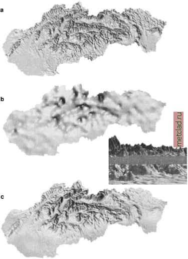Figure 7.11. Interpolation of precipitation with influence of topography: a) Input 500 m resolution DEM; b) precipitation distribution using bivariate interpolation by s.surf.rst; c) precipitation with influence of topography interpolated by s.vol.rst. Precipitation is displayed as a surface ( hills are high precipitation values). The insert shows elevation surface intersected by 700 mm precipitation isosurface

s.vol.rst in=precip3d cellinp=dem500 cellout=precip.topo \ zmult=50 segmax=700

The command gS.list allows you to list the volume raster files that are available. The continuous volume from 3D scattered point data can be created by interpolation to 3D raster using the IDW method implemented as s.vol.idw, or the RST method using s.vol.rst, with RST usually providing more accurate results. The mathematical description of the method, including the equations for computation of associated gradients and curvatures, is in the Appendix B. Trivariate RST has similar properties and parameters as the bivariate version, so the principles described in the previous sections apply here as well (see for example impact of tension in 2D and 3D in Mitas and Mitasova, 1999).

To illustrate the volume interpolation, you can create a volume model of spatial distribution of the Chesapeake Bay nitrogen concentrations.

The horizontal resolution is defined as 500 m with g.region and the vertical resultion dres as 3000 m with gB.createwind, creating a volume with a single layer, starting at 0 m elevation and ending at 3000 m. The segmentation can be skipped by using segmax=7 0 0, because the number of input data points is only 435. The impact of topography on the resulting precipitation map is controlled by the vertical scaling parameter zmult, as well as by the resolution and smoothing of the DEM as demonstrated by Hofierka et al., 2002a. The resulting map precip.topo is a 2D raster map representing the precipitation. The 3D RST module internally computes a 3D (volume) precipitation function. When using the cellinp option, the precipitation values are extracted from the precipitation volume at the elevations given by the dem5 0 0 raster map (see Figure 7.11). You can experiment with tension, smoothing, and zmult parameters to get the best result. This approach captures a more complex, spatially variable relation between precipitation and elevation than the traditional methods that are based on statistical correlation.

7.3.7 Volmne and volume-temporal interpolation (ff)

GRASS provides some limited experimental tools for working with volume data. We describe the functioning tools here to encourage further development. Some of the prototype applications are demonstrated at the Spatial interpolation Web site.6 To illustrate the volume data processing tools we use the Chesapeake Bay nitrogen concentration data that can be downloaded from the related GRASS Tutorials Web site (see Endnotes), see also an example at the Multidimensional Spatial interpolation Web site. First, you need to set up a LOCATION based on the metadata and import the site file. Then define the 3D region using gS.createwind and gS.setregion, and you can convert the 3D point data (x,y,z,w) to discrete voxel representation with s.to.rastS:

Note that the site data should be in the correct 3D format: xyz#n %w1 and that the vertical resolution of the resulting grid is much higher than the horizontal resolution. Parameter zmult is set so that the vertical distances between the data points are of the same magnitude as the horizontal distances to ensure the stability of interpolation. See the Section 8.2.4 for various possibilities to visualize the results.

Similarly to the bivariate version, trivariate RST can compute a number of parameters related to the gradients and curvatures of the volume model. An experimental version of RST interpolation for 4D data (volumes changing in time) s.volt.rst is also available for update and further development.

7.3.8 Geostatistics and splines

As we have described in the previous sections, GRASS provides fully integrated spline interpolation and a wide range of geostatistical tools, including kriging through the link with Open Source geostatistical software (see Chapter 13). Because the relation between splines and kriging is a frequently asked question, we provide here a brief explanation.

Several authors (e.g., Wahba, 1990; Cressie, 1993) have demonstrated that splines are formally equivalent to universal kriging with the choice of the co-variance function determined by the smoothness seminorm (also called roughness penalty). Therefore, many of the geostatistical concepts can be exploited within the spline framework.

Kriging assumes that the spatial distribution of a geographic phenomenon can be modeled by a realization of a random function and uses statistical techniques to analyze the data (drift, covariance) and statistical criteria (unbiased-ness and minimum variance) for predictions. However, subjective decisions are necessary (Journel, 1996) such as judgement about stationarity, and choice of a function for theoretical variogram (variogram model). Kriging is therefore successful for phenomena with a strong random component and/or for the problems where estimation of statistical characteristics (uncertainty) is the key.

Splines rely on a physical model with flexibility provided by change of elastic properties of the interpolation function. Often, physical phenomena result from processes which minimize energy, with a typical example of terrain with

To limit the interpolation to the water body, import the shoreline data chesapeakeshore.ascii using v.in.ascii and create a mask for the Bay using v.to.rast. Then you can interpolate the masked volume using s.vol.rst: