
|
|
|
|
Главная --> Промиздат --> Map principle 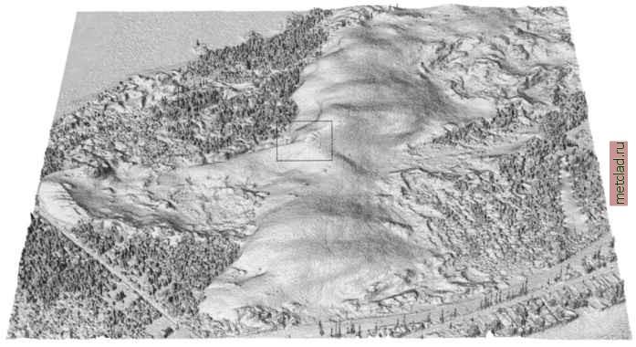 Figure 7.9. LIDAR data interpolated at 1 m resolution using the default settings of s . surf. rst. The rectangle is the area used in the previous figure illustrating the oversampling. Data are courtesy NOAA. NASA, and USGS (see the endnote of this chapter) 7.3.5 Surfaces with faults () By definition, spline is a smooth function and it has always been regarded as a tool for interpolation of smooth surfaces. However, RST can represent sharp edges or rough surfaces very well, if these features are sufficiently described by the data, as we have demonstrated in the previous section for LIDAR (see for example Figure 1.9). To create models of surfaces with complex faults pre-defined as vector lines, we can combine s.surf.rst with GRASS masking tools. We illustrate the approach using an elevation surface with a deep gully which was surveyed in the field (the data are available at the GRASS Tutorials Web site5). First, the points defining the fault need to be extracted from the measured elevation data, based on their attributes. We can format them as a GRASS ASCII vector line (see Chapter 6) using UNIX text processing tools. Then, we will import this faultline from a file gully.ascii, convert it to a raster, and use it as a mask to separate the gully area from the rest of the terrain: v.in.ascii gully.ascii out=gully v.support -r gully v.to.rast gully out=gully.mask Use the UNIX text tools to separate the points defining the gully (faultline and gully bottom) and the hillslopes, import them as point files elev.gully and elev.nogully, and interpolate with RST as follows: s.in.ascii elev.nogully input=nogully.ascii s.in.ascii elev.gully input=gully.ascii #interpolate without gully: s.surf.rst elev.nogully elev=elev.nogully #interpolate only gully: s.surf.rst elev.gully elev=elev.gully mask=gully.mask Use a mask for the gully to avoid unnecessary interpolation on the hillslopes where we do not have any gully data. The surfaces are finally merged using map algebra to create a single surface with faults (Figure 1.10): r.null gully.mask setnull=0 r.mapcalc elev.fault=if(gully.mask,elev.gully,elev.nogully) nviz elev.fault 7.3.6 Adding third variable: precipitation with elevation Multivariate interpolation is a valuable tool for incorporating the influence of an additional variable. For example, to interpolate precipitation with the influence of topography, the trivariate version of RST s.vol.rst can be used. 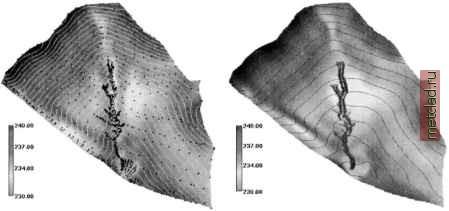 Figure 7.10. Interpolation of a surface with fault representing an edge of a gully. Given field measured data are shown as black dots The approach is similar to the one proposed by Hutchinson and Bishop, 1983, and it is described in more detail by Mitasova et al., 1995, and Hofierka et al., 2002a. The approach requires 3D precipitation site data (x,y,z,p) and a raster DEM. The result is a precipitation raster map computed as an intersection of the precipitation volume model with the elevation surface. As an example we use the computation of long term mean annual precipitation in Slovakia using the data from over 400 meteorological stations and a 500 m resolution DEM, described in detail by Hofierka et al., 2002a (the data are available for download on the GRASS Tutorials Web site, see Endnotes). The input site data precip3d include 3D coordinates for each meteorological station and mean annual precipitation as a floating point attribute, while the dem50 0 DEM is provided as a 500m resolution raster (Figure 7.11a). The output is a 2D raster map representing precipitation called precip.topo (Figure 7.11c). The 2D region should be set to the resolution of the input DEM. The module also expects that a 3D region is defined. To create it within your current MAPSET, you have to run the g3.createwind script. To ensure that the interpolation is performed only for the area of the Slovak republic, define the mask using the provided raster file mask. The resulting 2D precipitation raster map can then be computed by s.vol.rst: g.region rast=dem500 -p gS.createwind t=3000 b=0 dres=3000 g.copy rast=mask,MASK
|