
|
|
|
|
Главная --> Промиздат --> Map principle 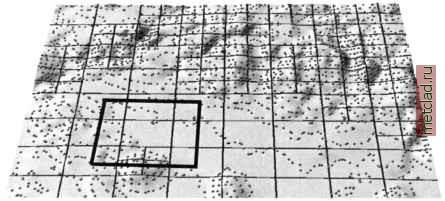 Figure 7.7. Segmented processing of large data sets smooth connection of segments for very low tension. The number of points in the segment is controlled by segmax, the number of points used for interpolation (within the segment and its neighborhood) is controlled by npmin. Default values for these parameters usually work, in case that the segments are visible, npmin should be increased. Note that while s.surf.idw uses 12 given points for computation of a grid value, s.surf.rst uses at least npmin points with the default npmin=2 0 0. If the points are dense and homogeneously distributed (as is often the case with LIDAR data), both segmax and npmin can be set to lower values, leading to substantially faster computation. The IDW computes a new function for each grid point, while RST uses the same function for all grid points within one segment. Automatized collection of data points, typical for the current digitizing and mapping technologies, leads to substantial oversampling. Therefore, the most effective tool for speeding up the computation is the reduction of data points to the minimum necessary for a given accuracy and resolution. The density of points used for interpolation in s.surf.rst is controlled by the parameter dmin representing the minimum distance allowed between the data points -points that are closer to each other than this distance are considered identical and not included into interpolation. As the LIDAR data are becoming increasingly available, we use them to explain the issues related to large data sets and oversampling. Our test data set for a large coastal sand dune called Jockeys Ridge in North Carolina, USA, can be downloaded from the NOAA LIDAR Data Retrieval Tool (LDART) Web site3, where you can also learn more about the technology. Use LDART to 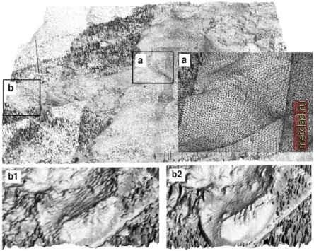 Figure 7.8. Surface created from raw LIDAR data by s.to.rast at 1 m resolution with lots of gaps. Insert a shows the input point data with overlapping swath in detail. Insert b1 shows detail of the surface created by s.to.rast at 3 m resolution with some loss of detail. Insert b2 shows detail of a surface computed by s.surf.rst at 1 m resolution with high level of detail select the North Carolina 1999 Fall mission and an area given by the following latitude-longitude coordinates: north: south: west: east: 35.96428 35.95287 -75.63844 -75.62579 LDART allows you to select a coordinate system, for example, you can choose UTM zone 18, with the horizontal datum nad83 and vertical datum navd88. Choose bin method none to get the point data. To import the data, first create a LOCATION (zone 18, north: 3980167, south: 3978908, west: 442433, east: 443573, resolution 3 m), then use s.in.ascii with the fd=, option. LIDAR point data create almost continuous coverage of the mapped surface; therefore, you can use s.to.rast to get a quick, rough view of the surface (Figure 7.8). You can do the transformation for 1 m and 3 m resolution as follows (Figure 7.8): g.region sites=lidar99 res=l -p s.to.rast lidar99 out=lidar99.sites.Im d.rast lidar99.sites.Im g.region res=3 -p s.to.rast lidar99 out = lidar99.sites . 3m d.rast lidar99.sites.3m With the 1 m resolution, there are lots of gaps in the surface. At the lower resolution, some detail was lost, and there are still a few gaps (Figure 7.8). To interpolate a high resolution DEM, we set the resolution to 1 m and interpolate with RST (Figure 7.9): g.region res=l -p s.surf.rst lidar99 elev=lidar99.def & With the default parameters, the interpolation can run for several hours so you should run it in background (<CTRL><Z>, bg). If you drape the given site data over the interpolated surface in nviz, you can see that the measured swaths of data overlap and the surface is significantly oversampled (see insert a in Figure 7.8). You can reduce the oversampling by increasing the parameter dmin from its default value of 0.5 meters (half grid cell size) to 1 or even 2 meters without losing too much detail. The points that are closer to each other than dmin are then skipped, leading to faster computation using a smaller number of sites. The most significant speed-up can be achieved by reducing segmax and npmin values to 20 and 100 respectively, because the high density of LI-DAR data does not require big overlaps in segments to achieve the continuity in the resulting surface. If you view the result in nviz (see Figure 7.9), you can see the excellent representation of the sharp dune crests and slip faces, even without defining them as breaklines, thanks to the high density of data points. The default values for tension and smoothing preserve the noise produced by laser scanning; to reduce this noise, use higher value of smoothing. In case of millions of data points exceeding the available RAM, swapping can be avoided by splitting the data into several overlapping strips, each interpolated separately and then patched together (overlap ensures smooth connection). The segmented processing as well as the possibility of splitting the computation into overlapping strips makes the module relatively easy to adapt to parallel processing. The experimental parallel version of s.surf.rst developed by Christoph Troyer is available at the NCSU GRASS contributions Web site.4
|