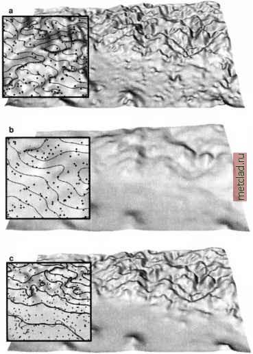Figure 7.6. Impact of constant and spatially variable smoothing: a) tension=40 and smooth-ing=0.0: surface passes exactly through the data points, but overshoots may be present; b) tension=40 and smoothing=10.0: surface is very smooth and does not pass exactly through each data point; c) tension=40 and smoothing is 0.1 in the mountainous area and 10.0 in the lowland. Compare these results with the surface interpolated with default parameters tension=40, smoothing=0.1 in Figure 7.3c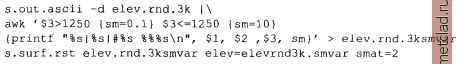

The module s.out.ascii pipes the sites to the awk program which sets the internal variable sm according to the third parameter $3 as piped from s.out.ascii. In our case, this third parameter is the elevation. The next code section within awk prints formatted (printf() function) GRASS internal sites format. The %s are needed to print the values stored in the variables $1, $2 and $3 as well as sm into this formatted string. This procedure is done for every line in the sites file and the output is redirected into a new sites map elev.rnd.3ksmvar which has an additional column containing the variable smoothing parameter. In the example with the variable smoothing, surface in the mountains (elevation greater than 1250) is identical with the one obtained from the default settings, on the other hand, the surface in the lowland is much smoother (Figure 7.6c).

7.3.3 Estimating accuracy

Several measures can be used to estimate accuracy of spatial interpolation. The module s.surf.rst computes deviations of the resulting surface from the given site data that can be output to a site file devi for further analysis. For example, you can compare the deviations of the surfaces generated by the RST default settings (smoothing 0.1) and with a smoothing of 10 by adding the output of the deviation file to interpolation and then computing the summary statistics as follows:

g.region rast=elevation.dem -p

s.surf.rst elev.rnd.3k elev=elevrnd3k.def devi=elev.def.devi s.surf.rst elev.rnd.3k elev=elevrnd3k.smlO smo=10\

devi=elev.smlO.devi

s.univar elev.def.devi [...]

standard deviation 3.13887 mean of absolute values 2.17833 [. . .]

s.univar elev.smlO.devi [...]

standard deviation 21.7113 mean of absolute values 15.3396 [...]

r.info elevrnd3k.def [. . .]

... rmsdevi=3.138342 [. . .]

r.info elevrndSk.smlO [...]

... rmsdevi=21.707725 [. . .]

When you compare the standard deviation and the mean of absolute values of deviations, you can clearly see that the surface with the lower smoothing is closer to the data points than the surface with the high smoothing. Your values of deviations may be slightly different from those published here because your input file, generated by a random procedure, will be slightly different too. Even if the devi file is not defined, the standard (root mean square) deviation is written into the history file of the resulting raster, along with the minimum and maximum of the values at the given points and in the interpolated raster. Note that the interpolated minimum and maximum values are usually higher or lower than those at the given points, due to the smoothing, especially if the interpolation is performed outside of the area covered by the input data set. The contents of the history file can be retrieved by r.info.

The predictive error of the RST interpolation for the given set of parameters can be estimated by a cross-validation procedure (Mitasova et al., 1995) implemented in an experimental version of s.surf.rst.cv (available at the NCSU Web site.2) The method is based on removing one data point at a time, performing the interpolation for the location of the removed point using the remaining samples, and calculating the residual between the actual value of the removed data point and the estimate for this point obtained from the remaining samples. This procedure is repeated until every sample has been, in turn, removed. The overall performance of the interpolator is then evaluated as the root-mean of squared residuals. Low root-mean-squared error (RMSE) indicates an interpolator that is likely to give more reliable estimates in the areas between the data points. The cross-validation can also be used to find optimal interpolation parameters by minimizing the RMSE (Mitasova et al., 1995, Hofierka et al., 2002a).

7.3.4 Interpolating large data sets

Digitized contours or LIDAR (Light detection and ranging) elevation data sets can have over a million data points with the resulting DEMs with thousands of rows and columns. To support processing of such large data sets, s.surf.rst and s.vol.rst were implemented with a segmented processing procedure. The segmented processing is based on the fact that splines have local behavior, i.e., impact of data points which are far from a given location diminishes rapidly with increasing distance (Powell, 1992). The segmentation uses a decomposition of the studied region into rectangular segments with variable size dependent on the density of data points (Figure 7.7), using quadtrees for 2D and octtrees for 3D interpolation (Mitasova et al., 1995). For a given segment, the interpolation is carried out using the data points within this segment and from its neighborhood, selected automatically depending on their spatial distribution. Because tension inversely controls the range of influence of data points, this approach requires large neighborhoods to achieve