While the results may be satisfactory for many applications, it is worth exploring the full functionality of this module because it provides a number of additional capabilities, ranging from tuning the character of the resulting surface to computation of topographic parameters. Here, we discuss how to choose the parameters to optimize the spatial interpolation and evaluate its accuracy. In Chapter 12, we demonstrate the use of s.surf.rst for topographic (surface geometry) analysis.

To take the full advantage of the s.surf.rst, understanding the principles behind the method is important. The mathematical description is given in the Appendix B; here we provide only a verbal description with illustrations. The RST function minimizes a specific measure of surface smoothness (also called smoothness seminorm or roughness penalty) and simulates a flexible sheet forced to pass through the data points while minimizing its energy (Mi-tas and Mitasova, 1999, Wahba, 1990, Talmi and Gilat, 1977). Properties of this function can be controlled by the tension and smoothing parameters. See the difference in the impact of these two parameters illustrated by two animations at the Multidimensional Spatial Interpolation Web site1.

Tension parameter. Tension tunes the surface from a stiff plate to an elastic membrane (Figure 7.4, Mitasova and Mitas, 1993). For very high tension, the surface resembles a rubber sheet with cusps at the data points (Figure 7.4b, tension=160, default smoothing=0.1). For low tension, the surface behaves like a stiff (hard to bend) plate, creating a very smooth surface (Figure 7.4a, tension=10, default smoothing=0.1). Due to its stiffness, it can overshoot in the areas of sharp gradient change (especially if zero smoothing is used, as in Figure 7.6a); in that case, the program gives a warning and increase in tension or smoothing is suggested.

The role of the tension parameter can be also interpreted as a control of the range over which the given point influences the resulting surface. For the high tension, each point influences only its close neighborhood and the surface goes rapidly to trend between the points. This may create cusps around the data points (Figure 7.4b) or steps along the contours (Figure 6.7c). With very low tension, each point has a long range of influence, so it is suitable for interpolation of areas with relatively flat terrain with data points spaced far appart. On the other hand, it may cause visible segments in large data sets (see Section 7.3.4 for a solution). The default input parameters try to adjust the tension to a suitable value based on the analysis of the data point density; however, to fully optimize the tension a more complex procedure based on cross-validation may be used (see Section 7.3.3).

To explore the impact of tension (Figure 7.4), you can interpolate two different surfaces from the Spearfish random elevation data as follows:

s.surf.rst elev.rnd.3k elev=elevrnd3k.tlO ten=10 s.surf.rst elev.rnd.3k elev=elevrnd3k.t160 ten=160

You can compare these results with the surface computed with the default ten-sion=40 and smoothing=0.1 in our first example in the Figure 7.3c.

Because the tension parameter is scale dependent, it can have different values in different directions, supporting modeling of anisotropic surfaces and volumes (Figure 7.5, Hofierka et al., 2002a). Two additional parameters, angle and scale, were added to s.surf.rst in GRASS 5.3 for computation of surfaces with uniform anisotropy, where the new parameters theta and scalex represent the direction and ratio (scaling) of the anisotropic features.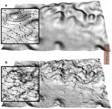

Figure 7.4. Tuning the character of interpolated surface by tension parameter: a) tension=10, smoothing=0.1 leads to a smooth surface with low level of detail useful for modeling major trends; b) tension=160, smoothing=0.1 leads to a surface with cusps (little peaks and pits) in data points, but it is smooth in between (as opposed to IDW). Note that the same smoothing was used in both examples. Compare these results with the surface interpolated with default parameters tension=40, smoothing=0.1 in Figure 7.3c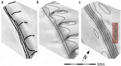

Figure 7.5. RST interpolation of a beach surface surveyed by Real Time Kinematic GPS:

a) given data points; b) default parameters in s.surf.rst; c) anisotropic tension with angle

theta=160 degrees and scaling scalex=0.25

Smoothing parameter. The functionality of smoothing can be illustrated using springs attached to the pins representing data points. The higher the smoothing the softer the springs and the more is the surface allowed to deviate from the data point in its effort to minimize its energy. GRASS implementation supports the spatially variable smoothing parameter - each site can have different softness of its spring. The interpolation function will pass exactly through the data points that have smoothing set to zero. Uniform smoothing is given as a constant parameter smooth, while variable smoothing is given as a floating point attribute in the site file. Smoothing is important when using low tension to prevent overshoots, as well as for removing the noise which may be present in data.

To explore the impact of smoothing, you can interpolate 3 surfaces from the Spearfish random site data using the default tension ten=40 and the smoothing set to a) smo=0, b) smo=10, and c) to spatially variable values with smo=0.1, if z > 1250 and smo=10 when z <= 1250 (Figure 7.6, see Figure 7.3c for the result with the default smoothing=0.1):

s.surf.rst elev.rnd.3k elev=elevrnd3k.smO smo=0 s.surf.rst elev.rnd.Bk elev=elevrnd3k.sml0 smo=10

You can use awk to add the variable smoothing to your site file within the directory site lists in your MAPSET: