
|
|
|
|
Главная --> Промиздат --> Map principle 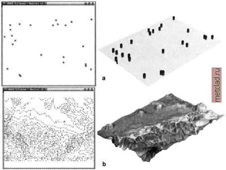 Figure 7.2. Conversion of site data to raster for: a) discrete phenomenon - archaeological sites; b) continuous phenomenon - elevation Voronoi polygons. This method is suitable for transformation of qualitative site data when the condition of continuity is not appropriate. The site attribute is simply assigned to all cells within its natural neighborhood defined by a voronoi polygon (Fortune, 1987). The module s.voronoi generates these polygons as a vector map layer with each polygon carrying the site attribute. You can then transform this vector map layer to a raster using v.to.rast, resulting in a surface composed of discontinuous, horizontal patches (see Figure 7.3 a). The procedure, using the random samples of Spearfish elevation data (see Section 7.1.2) starts with modification of the elev.rnd.3k site file in the site lists directory in your MAPSET: 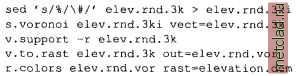 The module s.voronoi expects the values as category numbers, therefore we have used the sed command to change the prefix % to #. The resulting 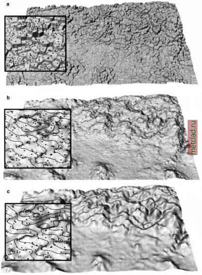 Figure 7.3. Interpolation methods available in GRASS and the resulting surfaces: a) s.voronoi, b) s.surf.idw, note the small peaks and pits around the data points, c) s.surf.rst. The surfaces are interpolated from the 3000 random samples of the Spearfish 30 m DEM Regularized Spline with Tension (RST). The method computes the values at grid points using a function which simulates a thin flexible plate passing through or close to the data points (Figure 7.3c). It is the most general and accurate method available in GRASS but it may require tuning of parameters to achieve optimal accuracy. Optionally, it also computes topographic parameters and partial derivatives of the modeled surface (see Chapter 12). The bivariate (2D) version is called s.surf.rst and the trivariate (3D) version is s.vol.rst. There is also a quad-variate experimental version available (e.g., for 3 spatial dimensions and time) called s.volt.rst for those who are interested in development of multivariate interpolation capabilities. The method, its properties and examples are described in more detail in the following sections. 7.3.2 Interpolating with RST: tuning the parameters Bivariate Regularized Spline with Tension (RST, Mitasova and Mitas, 1993, Mitasova et al., 1995, Mitas and Mitasova, 1999) is implemented in GRASS as s.surf.rst. To interpolate the Spearfish elevation random sites elev.rnd.3k (generated in Section 7.1.2) to a raster map layer elevrnd3k.def, we can simply run the module with its default settings (Figure 7.3c): g.region res=30 -p s.surf.rst elev.rnd.3k elev=elevrnd3k.def raster depends on the spatial distribution of input data. For example, the raster generated from contour points is quite different from the one generated from randomly distributed samples of the same surface (compare Figure 7.3a and Figure 6.7a). These figures clearly demonstrate that voronoi polygons are not a good choice for continuous fields, but they may be appropriate for numerous applications in ecosystem studies or geomarketing. Inverse distance weighted average (IDW). This approach calculates the value for each grid point as a weighted average of values at the n closest sites (Burrough and McDonnell, 1998, see the equation in Appendix B.8). In the GRASS module s . surf.idw weights are inversely proportional to a power p = 2 of distance and the default n = 12. It is a simple approach, however, the results are less accurate compared to other methods such as splines, krig-ing or multiquadrics (Mitas and Mitasova, 1999). Often the method does not reproduce the local shape implied by data and produces local extrema at the data points (Figure 7.3b, also noticeable as small circular contours around the given points). The module is useful for rough interpolation of smaller data sets, especially at lower resolutions, when the density of points is higher than the density of the resulting grid points. The Figure 7.3b was created by: s.surf.idw elev.rnd.3k out=elev.rnd.idw
|