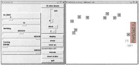Figure 7.1. Selecting a subset myarchsites.subl of site data myarchsites using d.siter, with categories 5-15 and northing > 4920429

To select subsets of site data with given coordinates, attributes, or categories use d.sites.qual. Its TclTk version d.siter allows you to display a subset of site data interactively, based on selected ranges of coordinates and/or attribute values. An example of using d.siter is in the Figure 7.1. Subsets defined by selected ranges of attributes may be visualized using various marker sizes, shapes, and colors. Subsets may also be saved to a new sites file. The command line version can be illustrated by the following example. It extracts a subset of sites from the map archsites with category numbers 5-15 that are located north of the given y (northing) coordinate:

d.sites.qual archsites rules=Cl.5-15,D2.ge.4920429 \ out=archsites.sub2

The subset is stored in a new site file called archsites.sub2a. You can find more examples of the rules syntax in the d.sites.qual manual page.

You can also use nviz to view your site data draped over a surface or in their 3D position (see Chapter 8).

To create a subset of sites located within a given subregion (defined for example by d.zoom), you can use the module s.mask with any raster with non-NULL cells: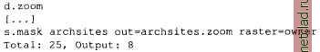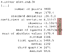

You can run r.univar elevation.dem to compare the result with the basic statistical measures of the original data. Please refer to Appendix B for a list of basic statistical equations used to compute these measures. Further statistical analysis can be performed using additional GRASS sites commands, such as s.normal which supports computation of 15 different normality tests for a selected site attribute. The module s.qcount provides a test for complete spatial randomness using a quadrat method, while a sample semivariogram can be computed by s.sv. You can fit a semivariogram model to the sample semivariogram using the module m.svfit. However, these modules havent been thoroughly tested, so they should be used with caution.

Note that besides using R and gstat, you can always transform your site data to raster or vector representation and use the raster and vector modules to greatly expand the possibilities for the point data analysis.

The module finds eight sites in the subregion and writes them into the new sites file. You can use the same command to find which sites are located within the 30 m cells representing roads:

s.mask archsites out=archsites.roads raster=roads Total: 25, Output: 2

7.2.2 Computing basic statistics

Simple statistical analysis of site data can be performed directly with several GRASS modules. For more sophisticated spatial statistics and geostatistics tools it is recommended to take the advantage of the bridge between GRASS and R, as described in Chapter 13, as well as by Bivand, 2000, or a link with gstat described in the same chapter.

Basic univariate statistics can be computed using s.univar. For example, for a random elevation data elev.rnd.3k created in the Section 7.1.2 you get:

7.3. TRANSFORMATION FROM SITES TO RASTERS AND SPATIAL INTERPOLATION

Depending on the type of data, the transformation of site data to the raster data model can be performed using two approaches (Figure 7.2):

for discrete phenomena, the transformation of site data to raster is done with s.to.rast. It creates an output raster file with the selected site attribute value in a cell where the site is located, while inserting NULLs elsewhere. If more than one site falls into one raster cell, the module will continue to import the sites and the last imported site value will determine the cell value;

if the site data represent sampling points of a continuous phenomenon, such as elevation, temperature, or chemical concentration, raster representation of this field should be computed by spatial interpolation.

For 3D sites, the discrete transformation to a 3D raster volume is performed using s.to.rastB and the spatial interpolation is supported by trivariate versions of the available interpolation modules, as described in the following sections.

7.3.1 Selecting an interpolation method

Spatial interpolation transforms site data to the raster representation using a function which passes through (or close to) the given sites. Because there exists an infinite number of functions which fulfill this requirement, additional conditions have to be imposed, leading to a number of different interpolation techniques. GRASS offers interpolation functions which are based on conditions of locality (voronoi polygons, inverse distance weighted) and smoothness (splines). The methods based on geostatistical concepts can be applied by taking advantage of the link with the Open Source geostatistical tools (see Chapter 13). It is important to keep in mind that different methods, and often even the same method with different parameters, can produce quite different surfaces (see, for example, Figures 7.3, 7.4, 7.6). A good knowledge of the modeled phenomenon is needed to evaluate which one is closest to reality. Statistical measures of accuracy do not always ensure that the properties of the interpolated surface are adequate representation of the behavior of the modeled phenomenon.

Before interpolating in GRASS, it is necessary to set the resolution of the resulting map layer with g.region (see Section 4.1.2). Several modules can then be used to interpolate a raster map from scattered site data.