
|
|
|
|
Главная --> Промиздат --> Map principle functionality class functionality integration of geospatial data raster data processing vector data processing site data processing image processing visualization modeling and simulations temporal data support volume data processing links to 0\vin Source tools import and export of data in various formats coordinate systems transformations and projections transformations between raster, vector and point data nmdels spatial interpolation comprehensive map algebra surface, topographic and watershed analysis correlation, со variant analysis cost surfaces, shortest path, buffers line of sight, insolation landscape ecology measures expert system (Bayes logic) digitizing overlay spatial autocorrelation multidimensional, muIti-attribute site data model summary statistics site buffers multivariate spatial interpolation and surface analysis voronoi polygons, tri angulation processing and analysis of multispectral satellite data image rectification and orthophoto generation principal and canonical component analysis reclassification and edge detection radiometric correction 2D display of raster, vector and site data with zoom and pan 3D visualization of multiple surfaces with vector and site data 2D and 3D animations hardcopy postscript maps hydrologic, erosion and pollutant transport, fire time stamp for raster, vector and site data 3D map algebra volume interpolation and analysis volume visualization (isosurfaces) R-stats, gstat, PostgreSQL, UMN/MapServer, Vis5D GPS tools, GDAL Table 3.1. GRASS GIS functionality There, you can find the source code (portable version for all platforms) as well as the latest ready-to-install binaries for Linux, SUN, SGI, MacOS X and MS-Windows NT/2000/XP (requiring the Cygwin tools). For some GNU/Linux distributions, RPM packages are provided. After successful installation, the package grass5package bin.tar.gz may be deleted. Refer to the Chapter II for information on the GRASS source code, the CVS server and code compilation. 3.1.2 Database and command structure GRASS data are stored in a UNIX directory referred to as DATABASE (also called GISDBASE ). This directory has to be created with mkdir or a file- manager, before starting to work with GRASS. Within this DATABASE, the projects are organized by project areas stored in subdirectories called LOCATIONS (Figure 3.I). A LOCATION is defined by its coordinate system, map projection and geographical boundaries. The subdirectories and files defining a LOCATION are created automatically when GRASS is started the first time with a new LOCATION (see Section 3.2 for more details). Each LOCATION can have several MAPSETs (Figure 3.I). One motivation to maintain different mapsets is to store maps related to project issues or subregions. Another motivation is to support simultaneous access of several users to the map layers stored within the same LOCATION, i.e. teams working on the same project. For teams a centralized GRASS DATABASE would be defined in a network file system GRASS is also available on CD-ROM, from the FreeGIS project Web site2 and for MacOS X from OpenOSX Web site3. There is a fee for packaging the CD-ROM and for the customized installation software. On the Web site you will also find the GDP - GRASS Documentation Project , which makes it easier to find documentation, especially for externally developed GRASS-modules and various articles. These pages can be reached at: http: grass.itc.it/gdp/ Support for developers and users is provided by several mailing lists to which you can subscribe using a Web interface (see the relevant links under Support section at the GRASS sites). Besides the English language international mailing lists, there are also localized lists currently in Czech, German, Italian, Japanese and Polish. GRASS binary installation. The GRASS binaries are available for several platforms. You have to download the install script grassSinstall.sh and the GRASS package grass5package bin.tar.gz (the name depends on the platform). The installation itself should be done as user root . It requires only one step (check online for appropriate file names): 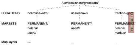 Figure 3.1. Organization of GRASS DATABASE, LOCATIONS and MAPSETs (e.g. NFS). Besides access to his own MAPSET, each user can also read map layers in other users MAPSETs, but he can modify or remove only the map layers in his own MAPSET. When creating a new LOCATION, GRASS automatically creates a special MAPSET called PERMANENT where the core data for the project can be stored. Data in the PERMANENT MAPSET can only be added, modified or removed by the owner of the PERMANENT MAPSET; however, they can be accessed, analyzed, and copied into their own MAPSET by the users. The PERMANENT MAPSET is useful for providing general spatial data such as elevation model write-protected to other users who are working in the same LOCATION. To import data into PERMANENT, just start GRASS with the relevant LOCATION and the PERMANENT MAPSET. This mapset also contains the DEFAULT WIND file which holds the default region boundary coordinate values. In all mapsets additionally a WIND file is kept for storing the current boundary coordinate values and the currently selected raster resolution. The internal organization and management of LOCATION, MAPSETs and map layers should be left to GRASS. Operations such as renaming or copying map layers involve several internal files and should always be done through GRASS commands (we discuss this in detail in Section 3.1.4). Non-GRASS interventions are acceptable only in exceptional situations and when one has a good understanding of GRASS internal structure. GRASS modules are organized by name, based on their function class (display, general, imagery, raster, vector or site, etc.). The first letter refers to the function class, followed by a dot and one or two other words, again separated by dots, describing the specific task performed by the module. Table 3.2 lists the most important function classes. The general syntax of a GRASS command which is called to run a module is similar to the UNIX commands: DATABASE
|