multiple flow direction (MFD) partitions the flow into 2 or more downs-lope directions, it is used by r.terraflow; r.topmodel, and the r.mapcalc flow implementation described in r.mapcalc tutorial (Shapiro and Westervelt, 1992);

bivariate (2D) flow used by r.hydro.CASC2D and an experimental module r.sim.water.

See Chapter 12 for examples of the practical applications of flow routing and comparison of the different approaches.

Watershed basin analysis is performed with r.watershed. As an example we calculate watershed basins from the elevation map in Spearfish region: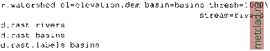

The threshold parameter is required to define the minimum basin size through cell numbers or overland flow units. The stream segment values correspond to the watershed basin numbers. Basins which are incomplete within the current region are omitted. This module does not require filling of depressions in DEM prior to its application because it uses shortest path algorithm to traverse the elevation surface to the outlet. In applications to new type of DEMs, based on LIDAR or radar surveys, this often leads to more accurate results compared to traditional methods.

For the flow accumulation and drainage direction analysis, the r.watershed module provides the option to use a binary depression (sinks) input map which contains lakes or other depressions in landscape that are large enough to store surface runoff. Such a depression map can be generated with r.fill.dir within two steps. First the DEM is filled, then the resulting filled DEM is subtracted from the original elevation map using r.mapcalc, with the result binarized on the fly using if-condition. The binary difference map is the depression map for r.watershed. In some cases, such as for the Spearfish elevation map, it is necessary to run r.fill.dir repeatedly (using output from one run as input to the next run) before all depressions are filled:

r.fill.dir in=elevation.dem elev=elevation.filll dir=directl r.fill.dir in=elevation.filll elev=elevation.f1112 dir=direct2 r.fill.dir in=elevation.f1112 elev=elevation.f1113 dir=direct3 r.mapcalc depressions.bin=if((elevation.dem - \ elevation.fill3)< 0., 1, 0) d.rast depressions.bin

D-infinity or vector-grid approach used by r.flow;

Because the D8 algorithm used in r.watershed is not suitable for dispersal flow on hillslopes, the module r.flow should be used for applications where overland flow pattern is needed. The program allows us to trace flow upslope or downslope and compute raster map layers representing flowline accumulation, flowline length, and a vector map for flowlines.

For computation of flow accumulation from massive DEMs that cannot be handled by r.watershed use the new r.terraflow module (Arge et al., 2003). This module is also useful for generating smooth flow pattern over hill-slopes using the MFD option with the possibility to switch to D8 single flow direction (SFD) routing for extracting the streams. You can learn more about flow tracing and watershed analysis in Chapter 12, which includes several applications related to land use management.

Geomorphology. The GRASS module r.param.scale extracts terrain parameters from a DEM with parameter feature. The morphometric features which are calculated are peaks, ridges, passes, channels, pits and planes. The resulting map depends on the moving window size. As an example, we extract morphometric features from the Spearfish elevation map:

r.param.scale elevation.dem out=morphology size=7 param=feature d.rast morphology d.legend -m morphology

The resulting map contains the above mentioned categories. If you plan to use this module for a serious research or applications we suggest that you read Wood, 1996, which provides detailed explanations and equations used in the module.

Sun illumination and solar energy maps. Many earth processes are influenced by the received solar energy. In environmental modeling, incoming radiation is needed as an input for evapotranspiration models; in urban planning and design, it is important for designing buildings and parks. For solar illumination effects and potential radiation calculations, GRASS provides two modules: r.sunmask to calculate a cast shadow map, and r.sun to calculate solar radiation (irradiance and energy) maps.

The module r.sunmask uses the SOLPOS2 algorithm from NREL (National Renewable Energy Laboratory) to calculate the position of sun in the sky for a given date, time, and a location on earth. You may use this feature for other purposes in case you need the sun position (r.sunmask provides a flag -s to calculate the sun position and exit then). For example, we can compute the cast shadow map in our Spearfish area for November 29, 2001 at 11:15h as:

r.sunmask -v elevation.dem out=shadow year=2001 month=ll\ day=29 hour=ll minute=15 sec=0 timezone=-7

As mentioned, the sun position and date calculation results from r.sunmask may be used as input for r.sun (Hofierka and Suri, 2002b, Suri and Hofierka, 2004), which requires the latitude and the day-of-the-year for the given location as input:

r.sun elevin=elevation.dem aspin=aspect slopein=slope lin=2.5\ alb=0.2 beam rad=b80 diff rad=d80 refl rad=r80 insol time=it80\ lat=44.4342 day=80

The radiation output maps b80, d80, and r80 contain direct (cloudless direct beam radiation), diffuse, and reflected radiation for the given day, respectively. The sunshine duration is recorded in it80 map. Optionally you can incorporate a shadowing effect of terrain using the -s flag. In mountainous and even hilly areas this can lead to very different results! Note that calculating the shadowing effect of relief can be computationally demanding.

Recall that you can get the map center coordinates for the current region with:

g.region -c g.region -1

The first flag -c reports these coordinates in the current coordinate system, while the second flag -l reports in latitude-longitude. See Section 12.2.3 later on for another application with r.sun.

Synthetic DEMs. To support terrain analysis, GRASS provides the module r.surf.fractal to create synthetic elevation models of selected characteristics (see Wood, 1996). The elevation models are created based on a given fractal dimension (Mandelbrot, 1983). This dimension D lies between the Euclidian dimensions 2 (plane) and 3 (volume), the closer D is to 3 the more rugged is the generated relief. We can compute a synthetic DEM with dimension 2.01 and display it as a shaded relief map as follows: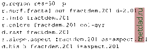

More structured elevation models can be obtained by increasing the fractal dimension D given as a parameter d.

Line of sight. The line of sight analysis creates a viewshed for a specific point in an area based on the digital elevation model. The module r.los generates a raster map output with the cells that are visible from a user-specified