find out which fire brigade is closer in terms of distance and potential speed to reach the fire. The result depends on the parameters used to prepare the input maps. Using r.what is probably the best idea, as we can directly enter the above coordinates of the fire brigades:

r.what roads.cost east north=590772.6,4926787.3

590772.6 I 492 6787.3 I I 7.8173332214 r.what roads.cost east north=608297.8, 4924206 . 0

6082 97.814 92 4206.01 17.7000617981

The result tells us that the fire brigade in Whitewood can reach the wildfire slightly faster (costs are lower) according to our definitions.

Of course we are also interested in getting the optimal route through the route network. The optimal routing module r.drain, which analyzes the cost surface, needs the coordinates of the fire brigades. Additionally we specify the flag -n to count the number of cells along the path (a simple indicator for the distance):

r.drain -n in=roads.cost out=spear.route\

coord=590772.6,4 92 678 7.3

d.rast spear.route

r.drain -n in=roads.cost out=white.route\

coord=608297.8,4 92420 6.0

d.rast white.route d.vect roads col=red

This delivers two path maps with accumulated numbers of cells, indicating the distance. Precise distance measure could be done by converting the raster lines to vector lines and generating a related line length report.

Note that r.cost only calculates along non-NULL values. In case that a starting point falls into a NULL area in the input map, you have to replace the NULL values with something meaningful for that application (in the above example a minimum speed). Either use r.mapcalc with an isnull () function to replace the NULL values, especially when you want to replace the NULLs with another underlying map, or use the r.null module when replacing the NULLs with a single value.

In our example we did not take into account that Deadwood, the closest town to our wildfire, is located south-east of the area. Another drawback is that some roads that appear connected on the raster map do not cross in reality, for example, if there is an overpass over the highway.

Computing a distance map. To compute the shortest distance of each pixel from raster lines, such as determining the shortest distances of households to the nearby road, you can use cost surfaces with cost value 1. The calculation is done with r.cost as follows (example for Spearfish region):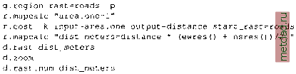

The map area.one is used as cost information, for calculating distances we use costs of 1. The distances are calculated from the roads network. Note that d.rast.num which prints the cell values as text labels into raster cells, only works when zooming into a map portion. The resulting distance map carries distance information in number of cells to the closest road. To calculate a real distance map (in meters), the cell values have to be multiplied with the cell resolution. In our example, we assume square pixels with identical resolution in north-south and west-east directions.

5.4.5 DEM and watershed analysis

Topographic analysis (or surface analysis) provides a wide range of parameters that describe the geometrical properties of the studied surface, such as:

a) summary parameters and profiles, for example volumes, surface areas, roughness, fractal dimension;

b) point parameters describing the geometry of the surface in the given point such as slope, aspect and different types of curvatures;

c) flow parameters based on integration along flowlines, such as slope length, upslope contributing area, watershed (basin), stream network;

d) ray tracing parameters based on lines (rays) emitted from or towards the surface, such as line of sight, insolation.

We will cover a subset of the above mentioned tasks in the following paragraphs.

Slope, aspect and curvatures. The module r.slope.aspect generates raster map layers of slope, aspect, curvatures and partial derivatives from a raster map layer of true elevation values. The slope values are calculated per default in degrees, or you may change the units to percentage using the parameter format. In case you are working in a coordinate system that uses feet (or units other meter), the module automatically converts the horizontal distances to meters. You must use parameter zfactor to convert elevation to meters to obtain correct values of slope, curvatures and derivatives. The aspect values represent the direction of flow (they point downslope) measured in degrees from east, increasing counterclockwise: 90° is north, 180° is west, 270°

is south and 360° is east. Additionally, you can calculate a profile curvature map (measured in the direction of the steepest slope) and a tangential curvature map (measured in the direction of the contour tangent). For exact definition of slope, aspect and curvatures see the equations in the Appendix B.3. Further explanation and applications of these parameters in relation to DEM quality assessment and modeling of processes is in Chapter 12. For general explanation of curvatures see, for example, Alexandrov et al., 1989 or Mitasova and

Hofierka, 1993.

The module computes topographic parameters based on approximation of the terrain surface by a second order polynomial. This leads to the computation of partial derivatives, needed for estimation of slope and aspect, as weighted averages of elevation differences in the 3x3 neighborhood of the given grid point (see Appendix B.3). The equations are also known as Horns formula (Horn, 1981). When applied to DEM represented by integer meters the aspect is biased in certain directions and reinterpolation to floating point DEM is recommended (see Section 12.1).

For example, to compute slope, aspect and profile curvature using the elevation map in the Spearfish data set simply run:

r.slope.aspect el=elevation.dem slope=slope asp=aspect\

pcurv=profcurv

Find more application examples of this command in Chapter 12.

Flow parameters and watersheds. Flow parameters are derived by flow-tracing and are integral rather than point parameters (the value at each cell is computed based on a sum of values from other cells - in our case along the flowpath). Flow routing is based on flowlines, which are curves perpendicular to contours with direction given by aspect (minus gradient). The basic flow parameters are:

watershed (basin) areas (upslope area for a given outlet);

stream network;

flowpath length (also hillslope length);

flow accumulation (also flowline density, used to compute upslope contributing area).

Numerous algorithms have been developed for flow routing, based on the approach for estimation of the steepest slope direction and distribution of water to the downslope cells:

single flow direction (SFD, D8) moves flow into a single downslope cell, it is used by r.watershed and r.terraflow;