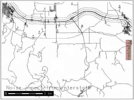Figure 5.6. Spearfish noise impact map from interstate (simple noise buffer model)

3 (250 m to 500 m) and 4 (500 m to 2500 m) which we have used for the buffering: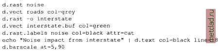

The resulting map shows only those residential areas which are influenced by the interstate according to the noise definition (see Figure 5.6). You can also query the map directly or print a report of affected residential area sizes (filtering all NULL values):

d.what.rast

r.report -n noise units=h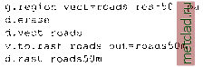

Note that the optional flag -a of g.region aligns the region boundary coordinates according to the resolution: the current region is slightly expanded to get a whole resolution number, in this case 50 m.

To store the location of the fire in a fire map, we use a sites module s.in.ascii which will be explained later in more detail in Chapter 7:

The echo command is a UNIX command to display a line of text. In this case we pipe the coordinates string to the module s.in.ascii which is effectively the same as storing the coordinates string into a text file and subsequently importing it. Next we have to reclass the roadsSQm map to obtain a map of potential specific travel time. This may be the inverse of the potential speed in km/h depending on the road quality. The reason to use the specific travel time instead of the speed is that r.cost considers high values as costly.

For the potential speed, you can use r.report to get the roads quality labels. Since reclassifications would only lead to integer maps, we use

5.4.4 Cost surfaces

Cost surfaces are raster maps showing the cumulative costs of moving between different geographic locations in an input raster map. Since GRASS 5.3 does not provide vector network analysis tools (but GRASS 5.7 will), this is an approach to reach similar functionality. Each raster cell in the input raster map will contain a value which represents the cost of traversing that cell. r.cost will produce an output raster map layer in which each cell contains the lowest total cost of traversing the space between each cell and user-specified points.

Let us start with an application - assume a wildfire in the Spearfish region at coordinates 597192E and 4915574N reported by an automated system. The fire was detected near an unimproved road in the Black Hills National Forest. Our task is to notify the fire brigade either in Spearfish (city north-west in our area) or Whitewood (village north-east in our area). The decision is influenced by two parameters: the potential speed to reach the destination depends on the roads condition and the distance to the fire. To solve the problem we have to calculate a cost surface .

The roads map is available as a vector map. We transform the vector map to a raster map with 50 m resolution. For that, we change the current resolution to 50 m, then transform the vector map to a new raster map:

r.recode to replace the road quality in roads50m with the specific travel time (which is a floating point value) in a new map. An example to understand the specific travel time: Considering 100 km/h as potential speed on the interstate for a fire brigade (label 1 in roads map), we calculate 1/100 = 0.01 h/km as specific travel time. To store these recode rules, we create a table roads.recode for all calculated values. This will replace the roads quality values with the specific travel time in a new map (refer to Section 5.3.5 for details):

1:1:0.0100:0.0100 2:2:0.0125:0.0125 3:3:0.0167:0.0167 4:4:0.0200:0.0200 5:5:0.0500:0.0500

Based on these recode rules, we generate a new map roads.travel:

cat roads.recode r.recode roadsSOm out=roads.travel r.report roads.travel

To make the map more meaningful, we define a new color table with high potential speed represented as green and the lowest potential speed as red with yellow in between: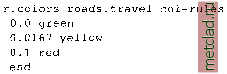

d.rast roads.travel d. sites fire col=red

To ensure that the full data range is covered, we define a lower specific travel time than the actual minimum value as green and a higher value as red. The value in the middle is taken from the above recode table.

The new map of specific travel time is the input to the cost surface module, which also requires the location of the wildfire. The costs to travel along the roads based on the inverse speed are then calculated from this location. Again, we redefine the color table for cost map, to make the map more communicative:

The fire brigade in Spearfish may be located at 590772.6E and 4926787.3N while for Whitewood it may be at 608297.8E and 4924206.0N. By visual inspection of the resulting cost map, mouse querying or using r.what you can