r.average base=fields cover=elevation.dem out=elevation.byfield d.rast elevation.byfield

To compute the average of values which are stored as category labels, we need to use the flag -c. In this case, the category label for each category in the cover map must be a valid number (integer or decimal). For example, to compute the average K factor (soil erodibility factor) for each field, we run:

r.average -c base=fields cover=soils.Kfactor out=Kfact.byfield d.rast Kfact.byfield

A module working in a similar manner is r.median which finds the median of values in a cover map within areas assigned the same category value in a user specified base map.

The area of a surface represented by a raster map can be computed by r.surf.area which calculates both the area of the horizontal plane for the given region and an area of the 3D surface estimated as a sum of triangle areas created by splitting each rectangular cell by a diagonal.

Volume calculation. To compute volume of an object defined by a surface (or its subsection defined by clumps) and a horizontal plane, you can use r.volume. In our example, we assume that a football stadium with a parking lot and related facilities will be built in Spearfish. For the construction the earths surface has to be excavated to a minimum depth of 5 m. To calculate the costs for the excavation work, we have to find the corresponding soil volume. The corners of the stadium area may be known from GPS measurements. To create a raster map of this area, store the coordinates of the stadium in the file stadium.txt in the following format (UTM coordinates for an area within Spearfish city):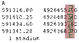

This will define a raster area by its corner points labeled as 1 stadium . As we operate only in Spearfish city, you may zoom into the city area before continuing. To zoom and import the raster polygon coordinates file, run: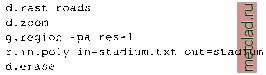

d.rast roads d.rast -o stadium

The flag -a aligns the region to the resolution, i.e. slightly extends it so that the resolution is a whole number. The resulting map contains the desired stadium area. We can now calculate the volume of the material that needs to be taken out (note that the map elevation.dem is only at 30 m resolution and an integer map, so the results will not be very accurate). Because we need to compute the volume only for a certain subarea, we will first set MASK to the area defined by the raster map stadium. Then, we normalize the excavation to have the bottom of the volume at zero elevation. This can be done easily by subtracting the desired minimum elevation from the DEM. We can find the minimum by running e.g. r.univar after masking all areas except the stadium: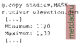

When using MASK the elevation statistics is calculated only for the stadium area. We store the portion of the DEM as defined by the current region into a new map and subtract the minimum height of the terrain and the desired excavation depth. Because part of the volume is below zero elevation now, we lift it up to achieve zero elevation as minimum. Then we can calculate the volume:

r.mapcalc excavation=elevation.dem - 1120 + 5 d.rast excavation r.univar excavation [. . .]

Minimum: 5 Maximum: 24

r.volume excavation Cat Average Data Number in clump Total 1 12.17 107461

# Cells Centroid Total

in clump Easting Northing Volume

8832 591375.50 4926425.50 107461.00

Total Volume = 107461.00

g.remove rast=MASK

The soil volume to be excavated for the stadium is roughly

Cross-category reports. We can easily generate reports for two or more maps which include occurrence of categories in the second map for each category in the first map. As an example, we can create a report which includes the areas in each land use category listed for each field owner category: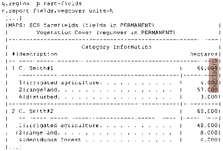

If you want to build a table using a set of maps, you can select them with g.mlist and send the list to the module in one line:

g.mlist type=rast pattern= soil* sep=, MAP=g.mlist type=rast pattern= soil* sep=, r.report map=$MAP

The characters have a special meaning in a shell (on the command line or in scripts). A command enclosed by these characters is executed and the message sent by the command can be stored in an environmental variable (in our case MAP) as above.

5.4.2 Overlaying and merging raster maps

As we have already mentioned, it is possible to overlay raster maps visually in the GRASS monitor using d.rast -o. However, to store such a raster map overlay in a new map, a different method is needed. To merge two maps into a single new map, use r.patch. It requires the input maps and a name for the new output map. The specified input map order determines the result: The NULL areas in the first map (which is on top of the virtual map stack) are filled with values from the second map and so forth for further maps. Overlaying or