in resolution, a check board structure may appear. On the other hand, the method is very fast and simple and has a special option for wrap-around interpolation of latitude-longitude rasters.

Resampling. GRASS uses automatic resampling when the region resolution is different from the resolution of the given raster map. Resampling can be also applied to a raster map by r.resample. When resampling from lower to higher resolution, the high resolution cells are assigned the same values as the cell within which they are located. When resampling from higher to lower resolution, the low resolution cell is assigned the value of the high resolution cell which is located the closest to its center (nearest neighbor). Resampling is designed for raster data which represent geometrical features, such as lines and areas (raster maps with categories). If applied to raster maps representing continuous fields, the resulting surface may have a checkerboard pattern (see Figure 5.3).

5.3.5 Receding of raster map types and value replacements

Sometimes we need to convert between different raster map types. The module r.recode has routines for conversion between every possible combination of raster type (e.g. INT to DOUBLE, DOUBLE to FLOAT, etc). The recoding is based on the rules which are read from standard input (i.e., from the keyboard, redirected from a file, or piped through another program). Standard output floating point raster data precision is FLOAT, with -d DOUBLE precision will be written. The general form of a recoding rule is:

To simply convert a raster between types, for example from INT to FLOAT, run the command with the following rule:

r.recode in=intmap out=fpmap << EOF

200:1500:200.0:1500.0

This will convert an INT raster map to a new FLOAT raster map with the same range of values. To convert the map from INT to DOUBLE while simultaneously changing the range of values we can use:

r.recode -d in=lntmap out=doublemap << EOF 200:1500:0.0005:0.000008

You will find additional alternatives for defining the rules in the r.recode manual page. Note that in the above examples we use another UNIX method to direct data such as the recode rules into the command r.recode. This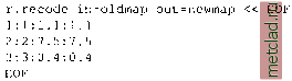

Each value appears twice because the module expects ranges for the old and new values to be specified. This value replacement method is often faster than formulating complex if conditions with raster map algebra through r.mapcalc.

5.4. SPATIAL ANALYSIS WITH RASTER DATA

A wide range of spatial analysis tasks can be performed using GRASS raster modules. Map overlay, generation of buffers, finding of shortest paths, and deriving topographic parameters can be combined to analyze complex spatial relationships. We describe some of the modules in the following section.

5.4.1 Map statistics and neighborhood analysis

To compute univariate statistics for a raster map use r.univar. It computes the number of cells, minimum, maximum, range, arithmetic mean, variance, standard deviation, and the variation coefficient. As an example, we apply it to the map elevation.dem:

g.region -p rast=elevation.dem r.univar elevation.dem [ . . . ]

Number of cells: 292317 Minimum: 1066 Maximum: 1840 Range: 774

Arithmetic mean: 1353.67 Variance: 31343.4 Standard deviation: 177.041 Variation coefficient: 13.0786 %

method is very convenient, especially for script programming. In the first line EOF (end of file) is specified, the module reads input unless the second EOF appears.

Value replacement. In order to replace existing cell values with different ones, you can again use the module r.recode. The formatting of the recoding rules is the same as described above. In the following example, the old values 1, 2 and 3 are replaced by 1.1, 7.5 and 0.4 respectively:

Please refer to Appendix B for equations. The area statistics for each category or floating point range is computed by r.stats, which we have already described in Section 5.1.6.

Neighborhood analysis. The neighborhood operators determine a new value for each cell as a function of the values in its neighboring cells. All cells in a raster map layer, except the cells at the map boundaries, become the center cell of a neighborhood as the neighborhood window moves from cell to cell throughout the map layer. The following neighborhood operators, with user defined sizes of the moving window, are available in r.neighbors (see Appendix B for equations):

average: the average value within the neighborhood;

median: the value found half-way through a list of the neighborhoods cell values, when these are arranged in numerical order;

mode: the most frequently occurring cell value in the neighborhood;

minimum: the minimum cell value within the neighborhood;

maximum: the maximum cell value within the neighborhood;

stddev: the statistical standard deviation of cell values within the neighborhood (rounded to the nearest integer);

sum: sum of cell values within the neighborhood;

variance: the statistical variance of cell values within the neighborhood (rounded to the nearest integer);

diversity: the number of different cell values within the neighborhood;

interspersion: the percentage of cells containing categories which differ from the category assigned the center cell in the neighborhood, plus 1.

As an example, we can compute a simple biodiversity map as follows:

r.neighbors vegcover out=veg.diversity method=diversity size=5 d.rast veg.diversity d.legend -m veg.diversity

You can experiment with different neighborhood window size to see its impact on the resulting map. Please refer to the manual page of r.neighbors for further details.

To find an average of values in a cover map within areas assigned the same category numbers in a base map, you can use r.average. For example, we can compute the average elevation for each field as: