5.3.2 Generating isolines representing continuous fields

If the raster data represent a continuous field, their vector representation is by isolines, or in the case of an elevation surface, contours. The module for generating isolines is r.contour. You can let GRASS determine the minimum and the maximum isoline values, and provide only the contour interval by the step parameter. To generate contours with a 100 m interval for our elevation.dem, we can run:

The vector topology is built automatically and the resulting contour lines are stored in the vector map contour100 which can be displayed using d.vect.

A related question is how densely the contour lines should be generated. On the one hand they should not hide an underlying map, on the other hand, the information content should be sufficient to get good representation of the surface. In case that there are no additional requirements on the contour interval, the optimal value (step parameter) can be computed by the following formula, developed by Imhof (in Hake and Grunreich, 1994:382):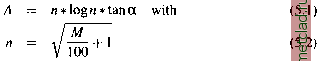

where A is the contour interval (vertical distance) [meter], a is the slope angle class depending of relief type [in degree], M is map scale [scale number]. The value of is selected based on the relief type:

mountainous region:

hilly region:

plains: a= 10°

For example, in a hilly region (a = 25°), for a map scale of 1:50,000 the optimal vertical distance is close to 15m. This value can be used in r.contour as step parameter. To find out the average slope for the selection of a you may calculate the univariate statistics of the slope map:

r.univar slope

The average slope is shown as Arithmetic mean . We will show later how to generate a slope map from the elevation data. The mathematical descriptions of the equations behind r.univar are given in the Appendix B.

The sites are shown per default as grey crosses which can be adjusted as described in Chapter 7 about site data processing. You can learn about additional methods for generating sites from raster data, such as r.random, in this chapter as well.

5.3.4 Interpolation of raster data and resampling

Transformation of a raster map layer to a different resolution is done internally whenever the region settings are changed. It is done by simple resampling which assigns the same values found in the original map to the cells in the resampled map, leading to a discontinuous surface. This approach has been designed for rasters representing classes. When changing resolution of rasters that represent continuous fields, interpolation should be used (Figure 5.3). Interpolation is also needed when filling gaps in merged raster data or when raster data are patchy and contain NULL values that need to be replaced to achieve continuous coverage.

Inverse distance weighted average (IDW) interpolation. Two modules for IDW interpolation of raster data are available: r.surf.idw and r.surf.idw2. Both modules compute the value at a grid point as a weighted average of a given number of neighboring grid points (default number of points is 12). The weight is depends on a distance between the computed grid point and the given point (see the equation in Appendix B.2). The main difference between the two modules is in the search method used for finding the neighboring grid points. The module r.surf.idw uses a more efficient approach and it also supports interpolation of data in geographic coordinates (latitude-longitude). A new resolution for the resulting raster map should be set using g.region before running the interpolation command.

5.3.3 Raster data transformation to sites

For some applications, it is useful to transform the raster map into a sites (points) map. GRASS provides the module r.to.sites for this purpose. Use the -a flag to output the cell values as a decimal attribute rather than a category number (which would be an integer).

The density of sites is controlled by the current region GRID RESOLUTION which you can adjust with g.region. To see how it works, we generate a sites map from the raster map transport.misc as follows: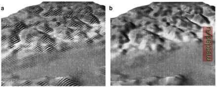

Figure 5.3. Difference between a) resampling and b) interpolation to higher resolution by RST

Regularized spline with tension (RST) interpolation. If there are large gaps in the raster data, it is advisable to use splines for the interpolation. If appropriate parameters are selected, the result will be much better than with the IDW method. The splines interpolation is available for raster, vector and site data, as r.resamp. rst, v.surf.rst and s.surf.rst. Because in GRASS 5.3 (which has been used in this book) the raster version r.resamp.rst was not sufficiently tested, we recommend transforming the raster map into sites, using r.to.sites or r.random (see Chapter 7.1.2 and Chapter 12) and using the s.surf.rst module. As in the previous case, the new resolution is selected using g.region before the module is executed.

Besides the interpolation, the s.surf.rst module can also calculate topographic parameters such as slope angles, aspect angles and curvatures (profile, tangential and mean). For details about the spline interpolation see the Section 7.3, Appendix B.2 and papers by Mitas and Mitasova, 1999, Mitasova and Mitas, 1993 and Mitasova and Hofierka, 1993.

When using interpolation it is important to check the quality of the resulting map, for example by computing the difference between the input and output raster maps and by viewing the associated slope and aspect maps to identify possible artifacts.

Bilinear interpolation. The bilinear interpolation is performed with r.bilinear. The interpolation function with constant gradient (a plane) is derived from the values of 4 points defining the cell centers in a given rectangular area. It can therefore be applied only to the raster maps with no NULL data values. The gradient of the interpolation function changes discontinuously across lines intersecting the cell centers of the input raster, so the method is useful only for small changes in resolution. For larger changes