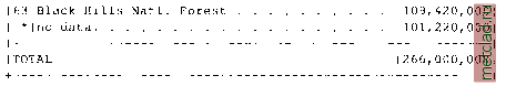r.stats -qan fields

1 640000.000000

2 600000.000000

3 300000.000000

[... ]

The -a flag allows us to print the area values in square meters related to a category, while -n suppresses NULL values. The flag -q suppresses printing of percent complete messages to standard output. Note that the area calculation depends on the raster resolution. The results from r.report and r.stats should be comparable.

However, we cannot use the output of r.stats as rules for reclassification of the fields map. Since we want to store the area values as category labels for each field we need to modify the output of r.stats, using a UNIX tool called awk. It is a pattern scanning and processing language which is very useful for modification of character strings and simple calculations with data stored in text files (see more details on how to use awk in the Appendix A). It allows us to modify a data stream on the fly:

r.stats -qan fields

1 640000.000000

2 600000.000000

3 300000.000000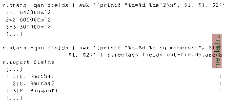

[...]

r.report fields.areas [. . .]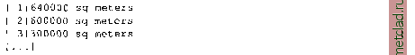

The redirection is done with UNIX piping which sends the output of r.stats directly to awk to do some formatting, then further on to r.reclass for generating the new map. If desired, you can copy the original color table from fields to fields.area with r.colors (see Section 5.1.1).

Clumping raster area features. For some applications we may need to create an individual category number for each raster area (polygon). For example, when the raster map includes several areas with the same soil type (assigned the same category number), we may need to distinguish each area, in case we are interested in computing the size of each area using r.report.

The module r.clump finds all areas of contiguous cell category values in the input raster map and assigns a unique category value to each such area ( clump ) in the resulting output raster map. Assume that we have a simple soils map with 3 soil types in 10 polygons. After clumping , we will have all 10 polygons numbered individually. Based on that you can assign the individual area sizes as shown above.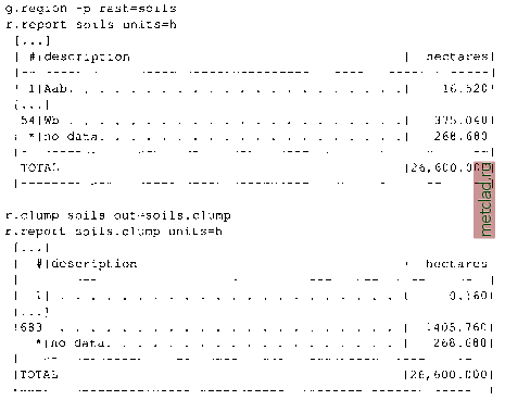

You can move around with cursor keys and select private ownership by entering 1 on the related line. Continue with <ESC><ENTER> and leave r.mask with another <ENTER>. Now, for any map that you display, you will see only the areas belonging to private ownership. Note that at the time of writing this book, the screen shown above listed no-data as 0, which is not correct and will be changed to NULL. Note that this MASK does not apply to vector and sites maps.

You can also generate MASK directly by creating a MASK file with r.mapcalc using if-condition as we explain later, or you can rename an existing binary raster map to MASK with g.rename.

While some soil names are assigned to several raster polygons in the original soils map, all raster polygons in the soils.clump map are numbered individually. This is useful, e.g. to calculate area sizes of the individual patches.

5.1.7 Masking and handling of no-data values

Raster MASK allows the user to block out certain areas of a map from analysis by hiding them from sight of other GRASS modules. Effectively, MASK is a raster map which contains the values 1 and NULL. Internally, the maps in use are multiplied pixel-wise with the MASK map. Those cells where the MASK map shows value 1 are available for display and computations while those masked by NULL are hidden. The map name MASK is a reserved filename for raster maps, if you have it in your MAPSET, it will be used as a mask in all raster operations.

To create a MASK, you need a base map. This map is used to select which values will represent the hidden and the active areas. As an example, we may decide to work only with areas belonging to private ownership , stored in the map owner. Now start the module

r.mask

and select menu entry 2 Identify a new mask . It requests a map name with Enter name of data layer to be used for mask . For our example enter owner here. A new screen appears showing the categories of the owner map.