i.target. Then assign coordinates for each map portion to the four map corners with i.points and the keyboard. Using i.rectify (again with a 1st order polynomial) the map portions are transformed into the projected LOCATION.

Once all scanned maps are transformed, the result can be checked in the projected LOCATION, leave the xy LOCATION for this. Now all individual

maps should be checked for their correct positioning and orientation, the base accuracy. Set the current region to the maximum (i.e. the default value) with:

g.region -dp

Open a GRASS monitor and display each map by:

d.rast ~o mapportion

The overlay mode (flag -o) allows us to overlay adjacent maps. With d.zoom you can now inspect whether distortions are visible between the maps. Next, cut off unwanted map borders and patch the portions to a seamless map. We explain this later on in Section 5.4.2.

4.1.5 Export

The export of raster data can be done in several ways. In GRASS 5.3 there is no general export tool available, this is planned for GRASS 5.7. Therefore a set of export modules exists which allows us to write various formats: GRASS ASCII (r.out.ascii), ARC/INFO ASCII GRID (r.out.arc), BIL (r.out.bil), BINARY ARRAY (r.out.bin), PPM (r.out.ppm), MPEG (r.out.mpeg), TIFF (r.out.tiff) and TARGA (r.out.tga).

As mentioned above, only the map portion of the current region will be exported. The export modules can be used on command line as well as interactively with menus. A few modules such as the ARC/INFO ASCII GRID, GRASS ASCII and PPM export modules optionally allow us to use UNIX piping, i.e. redirecting the data stream to another module. A piping example to produce a 8 bit GIF image is:

r.out.ppm elevation.dem out=- ppmquant 256 I ppmtogif>elev.gif

The result of r.out.ppm is directly sent to ppmquant to quantize the 774 elevation categories to 8 bit (256 colors), then to ppmtogif. The data transfer is done through standard out (stdout) indicated by - (dash). The GIF data stream resulting from ppmtogif is written to the elev.gif file. The produced GIF file is stored into the current directory.

Export to XYZ ASCII format. A common format for raster data exchange to other GIS is the plain XYZ ASCII format (i.e. x, y coordinates with the according z value). Unlike the GRASS ASCII raster export with r.out.ascii (which exports the data as an ASCII matrix), the following command produces a file with one line for each cell information, each line containing three columns (easting, northing, z):

r.stats -Ig elevation.dem nv= -9999 > altitudes.txt

The category label (attribute of the raster cell) is exported when using the -l flag, the optional nv parameter allows us to replace the NULL value with a different character or string.

4.2. VECTOR DATA

Line, area and point features can be represented in GRASS by vector data model. It stores the features geometry, attributes and topology. Three different vector types are used to store polygons (called vector areas in GRASS), lines (vector lines), and points (vector sites). The latter are convertible from and to the native GRASS sites data model.

4.2.1 GRASS vector data model

GRASS stores vector data using graphic elements (primitives) such as point, line, and area boundary (GRASS 5.7 stores additionally the centroid). Vector lines may consist of a single line (arc) or multiple connected lines (polylines). A closed ring of line segments defines a vector area. The end points of a vector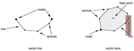

Figure 4.4. Vector types in GIS: vector line and vector area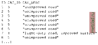

This is the logical structure of GRASS vector data category numbers and labels. In the GRASS database, the internal ID (left column) is not visible to the user.

GRASS vector data model includes topology, describing spatial relations between the graphic elements that define the feature location and geometry. With this type of data structure, the common boundary between two adjacent areas is stored as a single line, and shared nodes do not have to be duplicated. With topological information, it is possible to answer the following questions from a vector data set (Bartelme, 1995:18):

find neighborhood relationships between objects;

analyze if one object contains another object (island areas);

find intersections of objects;

analyze vicinity of two objects.

Detailed rules for digitizing vector data in a topological GIS are given in the digitizing section. For discussions on general computational geometry, see the book of ORourke, 1998.

line are called nodes, points along a line are vertices (see Figure 4.4). An area in an area is called island.

Vector lines and areas have attribute data assigned as a category number (attribute ID, also called CAT ID) and an optional category label (attribute text, also called CAT DESC). Both category number and category label may be shared with other vectors. Unlike in other systems, the internal unique vector ID is not visible to the user in GRASS 5.3. To assign attribute information to vector data, a label point, which links the attribute information to the geometrical data, is required. While vector lines have the label point positioned on the line, vector areas keep their label point within the area. GRASS is capable of managing only one attribute per vector internally, but a quasi infinite number when connecting the system to an external DBMS such as PostgreSQL. The internal structure of a roads map with vector ID, CAT ID and CAT DESC may look like this: