to be added to a so-called image group . This is simply a list of raster maps to be processed which is required to work with the i.* (image) modules. In our case, we only add this single map to the group list. To set up such an image group, run i.group either on the command line or interactively:

enter a name for this group, for example: mapscan. Hit <ESC><ENTER> to reach the main menu and confirm the new group name;

mark the scanned map with a x; hit <ESC><ENTER> to exit; leave the module with <ENTER>.

The next step is to define a target LOCATION (for example in UTM). For this purpose run i.target: select the group and enter the name of LOCATION and MAPSET (use list, <ESC><ENTER> to get a list of available

LOCATIONS and MAPSETS).

After having successfully set the image group and the target LOCATION, we now define the geographic reference points. They have to be set to tell the transformation module about a reference between the pixel coordinates of the scanned map and the related coordinates for every pixel in the projected LOCATION. Ideal points would be close to the four corners of the scanned map. It is recommended to read coordinates from the map using the grid printed on the map. The related coordinates can be typed in later during the assignment. GRASS provides a tool for convenient assignment of these geographic reference points using a mouse. To do that, first start a GRASS monitor with d.mon x0, then the module i.points. It will prompt for the image group (which just contains the scanned map), in our example the group mapscan . In the GRASS monitor, the scanned map has to be selected and then it will be displayed. In the graphical menu of i.points, you find a ZOOM entry. Using BOX you can enlarge the first corner of the scanned map. Make sure to zoom-in so that you can see each pixel well without losing the orientation on the map. Then, using a mouse click, select a point for which you have the coordinates from the paper map. Within the terminal window, GRASS asks you for the easting and northing of this point - type it in using the keyboard (delimited by a blank, see Figure 4.3). The same procedure has to be done for the other three corner points.

The quality of the point positioning can be directly analyzed using the ANALYZE menu entry. It calculates the RMS error after setting at least three reference points.4 It should not be larger than half of the true resolution of the scanned map as we have calculated above. The overall RMS error is a sum of all partial errors (one for every matching point). If it is too large, you can delete a point from the ANALYZE table (double click to toggle a point on and off) and select a new point. Once all four points are selected and assigned properly, leave i.points, and the points will be saved automatically.

Finally, we perform the transformation of the scanned map using the module i.rectify with 1st order transformation. After starting i.rectify, select a 1st order polynomial (as order of transformation ). This will perform the linear transformation (stretching and rotating). Next, enter a name for the scanned map for storage in the projected LOCATION (it may be identical). Now you have two options:

1. Use the current region in the target location

2. Determine the smallest region which covers the image

The first method is useful when you want only a subset of the scanned map (e.g. to cut off the borders). It uses the current settings of the target LOCATION. You have to be careful to preset the resolution and the current region according to the target coordinates of the scanned map. Otherwise you may obtain unwanted results. This method is useful after you get some experience.

The second method calculates the smallest region in the target LOCATION which covers the map. It may be sometimes larger than the DEFAULT WIND definition of the target LOCATION. Here you can adjust the boundary coordinates and the desired target resolution manually. When accepting the settings, you can directly set the current region of the target LOCATION to the new settings.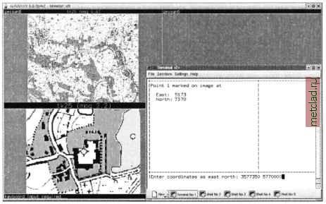

Figure 4.3. Geocoding of a scanned map with i.points

The module i.rectify then starts to transform the map. This may require some time, depending on map size, resolution, and hardware. As UNIX is capable of multitasking, you can continue working with GRASS, or even leave it, while the computation runs in the background. After the transformation has finished (at which point i.rectify sends an email), you can look at the new map in the target LOCATION. After restarting GRASS with the projected LOCATION and opening a GRASS monitor, the transformed map can be displayed with d.rast.

Quality control. The process described above takes a bit of time but leads to very accurate results when carried out with care. Quality control is always recommended, however. In combination with the zooming (d.zoom) the d.what.rast module allows us to check the coordinates of the four corner points used for the rectification. These should, of course, correlate with the equivalent points in the printed map. If the result is not satisfactory, we have to leave the target LOCATION and restart GRASS with the xy LOCATION. Now i.points can be called directly, because the group and target definition as well as the POINTS are still available. The accuracy can be increased by checking and improving the POINTS assignment. A new run of i.rectify is then necessary and the result should be checked again. The temporal xy LOCATION can be deleted after finishing the rectification as described in Section 3.1.4.

Note that this procedure is valid only for scanned, unreferenced maps. If you have digital data which are already geocoded and need to change the coordinate system, refer to Section 3.3 for an automated map transformation.

Seamless geocoding of multiple scanned maps. The transformation described in the preceding section can be used also for importing several scanned maps without gaps between boundaries. This is a way to import large maps which are too big for common scanners. The solution is to scan a large map in multiple parts. This is somewhat time consuming but useful if you do not have a large, expensive scanner.

The scanning of the map should be done with overlapping borders, to improve the identification of matching reference points. We assume that the map portions are available in a GRASS supported raster format. There also needs to be a target LOCATION, large enough to cover the complete map area.

Now set up a xy LOCATION as described above. Beware that the extent of the xy LOCATION has to cover the maximum extent of a scanned map portion. Import all map files into this xy LOCATION. Each portion will go into its own image group (so that it only contains one map) with i.group. Set the transformation target for all groups to the projected LOCATION with