Import of USGS SDTS DEM flies. The USGS SDTS DEM data sets consist of a number of files. Again, use r.in.gdal to import such a data set. Each DEM should have one file with a name like mapcatd.ddf which has to be specified as the import file. Projection and georeferencing information is respected.

Import of raster files in common image formats. You can directly import raster maps and images in the following formats: PNG (Portable Network Graphics), PNM (netpbm), uncompressed GIF, TIFF and JPEG. The module r.in.gdal will read these formats. As most of them do not provide projection information, you will have to apply the georeferencing manually. See the next paragraph how to do that.

Import of raster data without ancillary georeferencing flies. If you obtain a raster map in a common format such as TIFF, but without the related TFW file, you can update the geocoding manually. Of course you have to get the related georeference information from the data provider.

First, import the map with r.in.gdal. The lower left corner coordinates of the imported map will be at the origin of the LOCATION coordinate system, which is usually outside the study area. To georeference the map, the information in its header needs to be modified using the module r.support. After starting it, specify the map name. Then go through following dialog:

1 Edit the header? y. Rows and columns can be checked now. The values should be correct.

2 Pressing <ESC><ENTER> changes into the coordinates menu which looks similar to the LOCATION definition screen.

3 Now you have to update the boundary coordinates. Enter the correct coordinates and GRID RESOLUTION for this map by moving around with the cursor keys. Afterward hit <ESC><ENTER> to proceed.

4 The additional questions can be skipped with <ENTER>.

Further information on capabilities of the module r.support (e.g. changes of the color map) can be found in the GRASS manual of r.support.

4.1.4 Import and geocoding of scanned maps

In this section we explain rectification and georeferencing of a scanned map. For this procedure, it is important to be aware of the relation between geometrical length, scale and spatial extension. This general cartographical relation is also valid when transforming an analog map into a digital map. Because you will most likely be using a scanner (at least to create a backdrop map for the

vectorization within the GIS when you dont have access to a digitizer board), these terms are of great importance. Also, keep in mind the proper handling of copyright restrictions when scanning maps.

Determining scanning parameters. The relationship between distance in nature (ground truth) and corresponding length of a raster cell is determined by the scanning resolution. When working with toposheets, scanning resolution somewhere between 150 and 300 dpi is recommended. Of course the text labels on the map should stay readable. Depending on the number of colors in the map, the image can be scanned as color image with 256 colors. As an example let us assume a scanning resolution of 300 dpi. First we calculate the equivalent in centimeters:

mOdpi = 300

lines

= 118.11

lines

(4.1)

2.54cm cm

Suppose that the scale of the scanned map is 1:25,000. Thus, one centimeter on the map is equivalent to 25,000 cm in nature. Now we can calculate the distance in nature corresponding to the length of a raster cell:

distance in nature

25,000c-w

= 211.6-- =2.12 line

m line

(4.2)

scanned lines per cm 118.11 lines

The resulting value of 2.12 m is the spatial resolution of the map at the 300 dpi scan resolution. If you want the spatial resolution to be an integer, do the inverse calculation and adjust the scanning resolution accordingly.

Geocoding of scanned maps. After scanning the map, we store it in an external file. If needed, we can convert it to a GRASS supported format using gimp, display or xv which are available for many operating systems, as well as the netpbm tools3 which can be run on command line.

To geocode a scanned map, we first import it into a temporal xy LOCATION, assign related coordinates to a few (usually 4) known points, and rectify it into a target LOCATION using a specific GRASS module. Note that the projection of the target LOCATION must be identical to that of the scanned map. We recommend getting the four points from the paper map. The general idea is shown in Figure 4.2. We will be using image processing tools for geocoding which are also explained in Section 9.4.1.

First, we have to create a xy LOCATION with a region large enough for the imported map. If you do not know the number of rows and columns of the scanned map, you can find it using one of the above mentioned image viewers. Start GRASS and define a new xy LOCATION (rows and columns according to the size of the scanned map, GRID RESOLUTION is I pixel). It does not matter if you define the xy LOCATION larger; unused cells will not affect the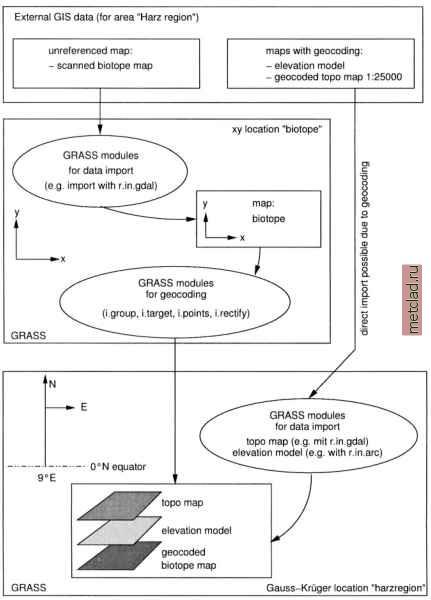

Figure 4.2. Sample workflow to import GIS data and to geocode scanned maps

allocated space on the hard drive. Now you can import the map using, for example, r.in.gdal.

After importing the map, the process is as follows (we need to use some commands here that will be the main topic in Chapter 9). The scanned map has