tem (NFS) without compatibility problems for raster data (from GRASS 5.7 onwards vector data is portable across different architectures). Internally, the integer format is called CELL, single precision floating point is called FCELL, and double precision floating point is DCELL.

The choice of the integer or floating point data depends on the users application. Their use can be described in general as follows:

Integer raster map layers: Rasterized geometric objects (points, lines, areas) are represented by non-continuous (discrete) fields. Each raster cell is assigned an integer value called category number. Each of the categories may have a label (usually a character string but a number can be used as well) describing the meaning or properties of these categories. Such category data as well as reclassified data and image data are stored in integer

format (GRASS CELL type).

Floating point raster map layers: Continuous fields such as elevation surfaces are often stored as floating point data (GRASS FCELL and DCELL types). It is possible to label these data by defining ranges of values (which can be interpreted as classes) and assigning each range a label (text or number).

3D floating point raster map layers: Raster volumes are stored as a voxel (volume pixel) data model (GRASS GRID3D type) designed to support representation of trivariate continuous fields.

Note that continuous field data can be represented in integer format (for example, some digital elevation models). This is a limitation of the data quality, and such data should be treated as continuous field representations! We will point out the related specific issues depending on the application later in this chapter and in Chapter 12.

GRASS also allows the user to create raster map layers by re-defining the classes as described in Section 5.1.5. In such a case, the reclassified map layer does not contain any data, but serves as a reference to another map layer along with a reclass table that is used to reclassify the values of the referenced raster map. From the users point of view such a map behaves as a regular raster map. Few GRASS modules do not work with reclassed maps; in such a case the module will report an error and suggest that the user generates a true copy of such a map (see Section 5.1.3).

4.1.2 Managing raster map resolution and boundaries

GRASS differs from other systems in the way it handles region (map extent) and resolution. While each raster map layer has its own resolution defined in its header, the operations with raster data are performed using the working

(or current) region and a resolution set by g.region. If the current region is smaller than the map extent of the raster that is being processed, the operation is applied only to the subset of the raster file defined by the current region. If the resolution is different, the raster is automatically resampled (see Section 5.3.4). This approach is also used when exporting raster data. It makes exporting subsets of raster maps very convenient, including export at a lower resolution. Note that the GRID RESOLUTION defined when setting up a LOCATION is the default region resolution and will be used only if the current region is set to the default region.

To adjust the current region to different values, you can use g.region. After starting the module, you get to the menu which allows you to modify the current region boundaries and resolution. If necessary, you can save the current region settings as a region file. This is sometimes useful when working on different subregions within the given LOCATION. This module can be efficiently used in the command line mode, for example:

g.region res=12.5

will set the resolution to 12.5 map units (e.g. meters). The region can be also defined from existing maps:

g.region rast=elevation.dem -p

which will adjust the current region according to elevation.dem. The flag -p additionally prints the current settings to the screen as follows (UTM pro-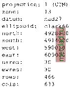

If you want to reset to the default region (boundary coordinates and raster resolution) of the LOCATION use the -d flag:

While the 3D capabilities are still in the development stage, we should mention at least briefly management of boundaries and resolution for volume data.

The 3D region is managed with gB.region or, with its command line version, gB.setregion, similar to 2D GRASS regions. If no 3D region exists yet, it must be created with gB.createwind. This module extends the 2D region definition by the third spatial dimension along with a user defined voxel resolution.

4.1.3 Import of georeferenced raster data

When importing raster data, we need to distinguish three general raster format types:

Binary image formats, which include only positive integer values (e.g., JPG, PPM, PNG etc.);

Binary raster formats: integer and floating point supported, both negative and positive values, single and multiple bands, single and multiple resolutions (such as ERDAS IMG, HDF, GeoTIFF etc.);

ASCII raster formats, which can have integer and floating point values, both

negative and positive (e.g., ARC-ASCII, ASCII-GRID, GRASS-ASCII etc.).

All common GIS raster formats are supported. Note that only a few of them (e.g., ASCII) handle negative and floating point values. When obtaining data, make sure to get information about the coordinate system (projection, datum, etc.). For some formats, the metadata are directly stored in support files which are read when importing the data.

Most raster maps can be imported with r.in.gdal. It requires the GDAL library1 which is included in the GRASS binary releases. It supports a wide (and growing) range of formats and is able to auto-detect them. When importing with this command, you can automatically extend the LOCATION definition by using the flag -e in case that the imported map is larger than the default region:

r.in.gdal -e in=d44103d7.tif out=d44103d7

If your data set does not contain projection information and you are sure than the data projection matches the projection of the LOCATION, the -o flag allows you to use the LOCATION projection information for the imported map.

When using the tcltkgrass user interface select: IMPORT ~> RASTER MAP Various formats . The opened window contains a button file which provides a small file manager for selecting the source file. A new name which represents the name in GRASS DATABASE has to be typed into the second line.