(B.19)

P = fx+fy, q = P+\

The steepest slope angle yand aspect angle ttare computed from gradient f - {fx,fy)(its direction is upslope) as follows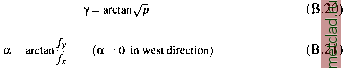

Sometimes we need to compute change of the surface in a direction given by an angle The directional derivative of the surface z = g(x,y) can be computed as

where (x,y) are the georeferenced coordinates, and a is aspect (given direction).

Curvatures. In general, a surface has different curvatures in different directions. For applications in geosciences, the curvature in gradient direction (profile curvature) is important because it reflects the change in slope angle and thus controls the change of velocity of mass flowing down along the slope curve. The curvature in a direction perpendicular to the gradient (tangential curvature) reflects the change in aspect angle and influences the divergence/convergence of water flow. Both curvatures are measured in the normal plane. Equations for these curvatures can be derived using the general equation forcurvature 1С of a plane section through a point on a surface (Rektorys, 1969, Mitasova and Mitas, 1993). The equation for the profile curvature is

The equation for tangential curvature at a given point is derived as the curvature of normal plane section in a direction perpendicular to gradient (direction of tangent to the contour line)

The positive and negative values of profile and tangential curvature can be combined to define the basic geometric relief forms (Krcho, 1973; Krcho, 1991; Dikau, 1989). Each form has a different type of flow. Convex and concave forms in gradient direction have accelerated and slowed flow, respectively, and convex and concave forms in tangential direction have converging and diverging flow, respectively.

Other types of curvatures, such as the principle, mean, or Gauss curvatures as well as curvatures in an arbitrary direction can be computed directly from the interpolation function.

Gradient and curvatures for volumes. Volumes can be modeled by a trivariate interpolation function in the general form of w = f(x,y,z). When this function is differentiate at least up to the 2nd order, the topographic parameters for volumes (3D) can be computed directly from its partial derivatives (Mitasova et al., 1995). First, we introduce simplifying notations for partial derivatives of this function: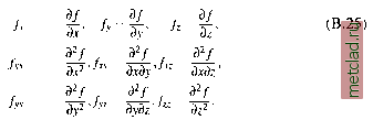

Volume topographic parameters are also derived from differential geometry, using additional independent spatial coordinate (z). Theoretically, such topographic parameters can be derived up to N-dimensional space (see Hofierka, 1997a). For a three-dimensional cartesian space these parameters have the following form: Size of gradient:

Direction of gradient can be defined by two angles. Horizontal angle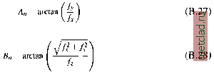

and vertical angle

The change of gradient size in its direction has the following form:

When we note principal curvatures in 3D cartesian space as then the Gauss-Kronecker

curvature K can by expressed as:

The mean curvature M is:

In cartesian system these equations can be expressed as follows:

fxzfyy fyzfxx I fxyfzz fxxfyyfzz ~ fxyfyzfxi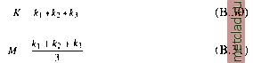

376 where:

Estimation of partial derivatives. To compute the above described equations for gradients and curvatures we need to estimate first and second order partial derivatives.

In the RST-based modules, partial derivatives of RST functions are used. First, several definitions are introduced

Partial derivatives for the bivariate RST basis function can then be expressed as follows:

/ 1,2 (B.43)

(B.44)

Ч / /

whereas the derivatives, according to y, are found easily from Equation B.44 by exchange of x to y. The mixed derivative is given by

These expressions for first and second order derivatives are used for the compulation of slope, aspect and curvatures in the modules s.surf.rst, v.surf.rst and r.resamp.rst. Optionally, the values of these partial derivatives are output by the module s.surf.rst when using the flag -d .