Appendix B

Selected equations used in GRASS modules

In this section we provide equations for selected GRASS modules, for those users who would like to have deeper understanding of the methods used in these modules and gain more confidence in advantages and limitations of the provided functionality. The equations are also helpful for those who would like improve or extend the modules.

While the number of modules for which we can provide the equations is currently limited we plan to extend this type of in depth description to other modules in future editions.

B.1. BASIC STATISTICS

Arithmetic Mean:

Arithmetic Mean is not unitless. Median:

The Median is the value below which 50% of the sample lie. To find the Median the data have to be ordered from smallest to highest. In case of an odd number of samples it is the middle value, in case of an even number of samples it is as half way between the two middle samples. Median is not unitless.

Variance:

Variance is not unitless.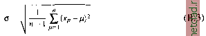

Skewness is zero for any symmetric distribution. A distribution with a long tail towards larger values has a positive skewness (left skewed, typical for remote sensing images, Schowengerdt, 1997: 118). Skewness is unitless and sensitive to outliers.

Kurtosis:

kurtosis -

(B.6)

Kurtosis is zero for a normal distribution. If a distribution has a positive kurtosis, than the peak is sharper than of a Gaussian distribution. Kurtosis is unitless and sensitive to outliers.

Covariance:

B.2. INTERPOLATION

Inverse distance weighted interpolation (IDW). The method is based on an assumption that the value at an unsampled point can be approximated as a weighted average of values at points within a certain cut-off distance, or from a given number m of the closest points (typically 10 to 30). Weights are usually inversely proportional to a power of distance (Watson, l992, Burrough, 1986) which, at an unsampled location r = (x,y), leads to an estimator

(B.8)

£Г=.г(г.)/г-г,Г I7.,l/r-r;/

where p is a parameter (typically p = 2, for more details on the influence of this parameter see Watson, 1992). GRASS modules use p = 2.

F(r) = £Mr,)

Regularized Spline with Tension. The function is a sum of a trend function and a radial basis function with an explicit form which depends on the choice of the measure of smoothness, for more details see Mitasova and Mitas, 1993, Mitasova et al., 1995:

Standard Deviation:

Standard Deviation is not unitless. Coefficient of variation:

Coefficient of Variation is unitless. Skewness:

The trend function Г(г) is given by

(B.IO)

Г(г) = 1 ;Л(г)

where { (r)} is a set of linearly independent functions (monomials) which have zero smooth seminorm. R{r, r-l) is a radial basis function with an explicit form which depends on the choice of weights for partial derivatives in the smooth seminorm. See Mitasova and Mitas, 1993, Mitasova et al., 1995 for the RST smoothness seminorm, which includes derivatives of all orders with their weights decreasing with the increasing derivative order.

RST can be generalized to an arbitrary dimension and the corresponding d-variate formula for the radial basis function is given by

rf(r,r,.) = Rd{\r ~ ryl) = Rdir) = p-8 Y(S,P) - g

(B.ll)

where r r - г;, 5 = (rf - 2)/2, and p = (q)r/2). Further, ф is a generalized tension parameter, and is the incomplete gamma function, not to be confused with semivariogram ( Abramowitz and Stegun, 1964). For the special cases d = 2,3,4 (s. surf.rst, s.vol.rst, s. volt, rst, respectively), the equation B. 11 can be rewritten as: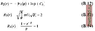

where C/r 0..577215... is the Euler constant, Ei(p) is the exponential integral function and erf(y) is the error function (Abramowitz and Stegun, 1964), while the trend function is a constant (M = 1):

r(x)=fli, d = г,ъ (B.15)

The coefficients A,j} are obtained by solving the following system of linear equations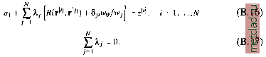

B.3. TOPOGRAPHIC ANALYSIS

Topographic parameters slope, aspect and curvatures are computed using the principles of differential geometry using the work by Krcho, 1973, Krcho, 1991 and Mitasova and Hofierka, 1993. Before deriving mathematical expressions for these parameters, using the basic principles of differential geometry, the following simplifying notations are introduced: