Before performing variogram modeling and kriging interpolation it is important to remove possible trends from data sets. As the zinc data probably contain a global trend, we apply a quadratic trend analysis (using Least Squares) to verify the situation: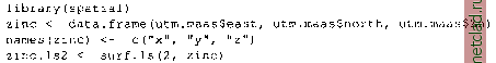

The function surf.lsO generates a trend model which is stored in object zinc.ls2. Next step is to evaluate a trend surface from this trend model by trmat.GO function. We can plot the resulting quadratic trend surface map zinc.trend2:

zinc.trend2 <- trmat.G(G, zinc.ls2) plot(G, zinc.trend2) points(zinc)

text{zinc$x, zinc$y, zinc$z, pos=l, cex=0.75)

Alternately we can also generate a cubic trend surface in a similar way:

zinc.ls3 <- surf.ls(3, zinc) zinc.trends <- trmat.G(G, zinc.ls3) plot (G, zinc.trend3) points (zinc)

text(zinc$x, zinc$y, zinc$z, pos=l, cex=0.75)

Finally we write the cubic trend surface map to GRASS as raster map:

rast.put (G, lname= soilsph.cts , zinc.trend3)

We can display this raster map with d.rast. 13.2.3 Using R in batch mode

R supports batch mode processing for a fully scripted usage. Within GRASS (maybe also scripted) geospatial data analysis can be automated. The desired analysis methods have to be stored in a text file (e.g. R.trendph.batch):

library(GRASS) G <- gmeta0

#load map:

soilsph <- rast.get(G, soils.ph , с(F)) names(soilsph) <- c( ph )

soils.ph.frame <- data.frame(east(G), north (G), soilsph$ph) soilsph$ph[soilsph$ph == 0] <- NA

Using GRASS with other Open Source tools (-f[-j names(soils.ph.frame) <- c( x , y , z )

#calculate cubic trend surface: library(spatial)

ph.ctrend <- surf.lsO, na . omit (soils .ph . frame) ) ph.ctrend.surf <- trmat.G(G, ph.ctrend)

#write plot to PDF: pdf ( trendSurf.pdf )

plot (G, ph.ctrend.surf, col=terrain.colors(20) ) contour.G(G, ph.ctrend.surf, add=T)

title ( Cubic trend surface of pH values in Spearfish region ) dev.off 0

#cleanup worlspace: rmdist = Is (all = TRUE))

The last command is needed to avoid that the loaded data are stored in the R workspace file .RData. Alternately the flag --no-save can be used when running the script. The other commands used here will be known from previous sections. This script is run within GRASS (Spearfish LOCATION) through

R batch mode:

grass53 /usr/local/share/grassdata/spearfish/user1 g.region -dpa res=100 R BATCH R.trendph.batch cat R.trendph.batch.Rout

The function (and eventual error) messages are echoed in the file R.trendph.batch.Rout for batch process verification. In the example above, a plot of the trend surface in PDF format is included. You should find this file in the current directory if no erroroccurs.

The next example shows a batch job which calculates the empirical cumulative distribution function (ECDF) of a given map. Here we make use of environment variables so that we can write the script as a general script for any filename. Store the script as R.ecdf.batch: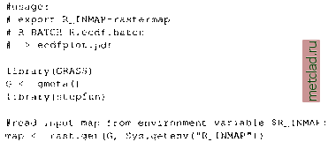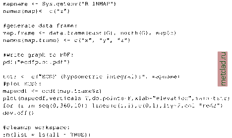

To run it you have to define the GRASS raster map name to be analyzed in the environment variable $R INMAP. We define it before starting the batch job (here for bash shell):

grass5 3 /usr/local/share/grassdata/spearfish/user1

g.region -dpa res=30

export R lNMAP=elevation.dem

R BATCH R.ecdf.batch

cat R.ecdf.batch.Rout

The resulting PDF file ecdfplot.pdf contains the graph showing the hypsometric integral of the input map (here: elevation.dem). When using above approach with environment variables, complex (pseudo) GRASS scripts can be written to extend functionality of GRASS by R.

13.3. GPS DATA HANDLING

The FreeGIS Web portal lists a set of programs freely available to handle GPS data. A basic problem to be addressed is the data transfer from GPS device to GIS including eventual datum transformations. These issues heavily depend on the GPS device. We only refer to a few software packages:

GPS Manager (GPSMan11) is a graphical manager of GPS data that makes possible the preparation, inspection and edition of GPS data in a friendly environment. GPSMan supports communication and real-time logging with both Garmin and Lowrance receivers and accepts real-time logging information in NMEA 0183 from any GPS receiver;