plot (zinc, scatter3d=T) quantile(zinc$data)

In Figure 13.8 the upper two plots are data locations, the lower two plots show the zinc data against the x and y coordinates. If the R extension scatterplot3d is not installed, the lower right plot will show a normal histogram instead of a 3D point data plot. The quantiles for the upper left plot are generated according to the results of the quantileO function.

The Maas river bank area can be retrieved from the already loaded maasmask data set which is a binary mask for the area. To generate a map with coordinates matching those of the binary mask (which is a R data vector only without coordinates), we export the map to GRASS and re-import it again. This will apply the related coordinates to the mask values:

str(maasmask)

rast.put(G, lname= riverbank , maasmask)

riverbank <- rast.get (G, riverbank )

names(riverbank) <- c( z )

str (riverbank)

plot (G, riverbank$z)

Here we are using the plot method for geospatial data as available through the R/GRASS environment (invoked through the G GRASS metadata object).

To plot the individually measured zinc concentrations into the Mass river bank map, we can use the points() and text() functions for setting the labels (pos=4 prints the labels right to the label point, cex=0.75 decreases the label font size):

points(utm.maas$east, utm.maas$north, pch=20, col= blue )

text(utm.maas$east, utm.maas$north, utm.maas$Zn,pos=4,cex=0.75)

titleCMaas river bank: zinc contamination [ppm] )

We see all sampling points labeled with the zinc concentrations measured as parts-per-million (ppm). The river Maas is at the north-west border of the project area, flowing in the north-east direction.

To find out whether the zinc concentration depends from the distance to the river we plot the variables Zn against d.river , both untransformed and transformed using natural logarithm (log() function in R). We can split the output screen into two parts with function par() and display two (or more) plots at the same time (we reset directly after plotting):

par(mfrow=c (2,1))

plot(utm.maas$d.river, utm.maas$Zn)

title( Maas river bank: zinc concentrations/distance ) plot(log(utm.maas$d.river), utm.maas$Zn)

title ( Maas river bank: zinc concentrations/ln\(distanceX) ) par(mfrow=c(1,1))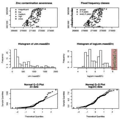

Figure 13.9. R/GRASS: Maas river bank data: zinc contamination analysis. Upper left: classes of zinc contamination severeness; upper right: flood frequency classes: 1=annual, 2=2-5 years, and 3=every 5 years; middle left: histogram of zinc concentrations [ppm]; middle right: histogram of logarithmic transformed zinc concentrations; lower left: QQ plots (Quantile-Quantile plot) of zinc data; lower right: QQ plots of log-transformed zinc data

The plot shows that moving from the river border, the zinc concentrations tend to decrease as expected.

We can look at the zinc data in more detail by analyzing the zinc concentrations for their severeness. First a new object is created with ordered data using the utm.maas object which contains the zinc concentrations. We generate five classes with defined thresholds, the example is based on the R/GRASS interfaces help pages: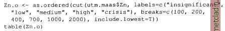

To plot the ordered zinc severeness data as a map with legend and title (compare Burrough and McDonnell, 1998:107), enter:

plot(utm.maas$east, utm.raaas$north, pch=codes(Zn.o), xlab= ,

ylab= , asp=l)

legend(x=c(270000, 270600), y=c(5652100,5652700), pch=c(l:5),

legend =levels (Zn.o)) titleCMaas river bank: zinc contamination severeness )

The codes() function is required to access the category numbers for the legend symbols. The legend is placed at certain coordinates into the map. The levels() function shows the different category labels for the legend. You can always call a function directly to see which results are generated (e.g. levels(Zn.o)). The map is shown in Figure 13.9.

Next we plot a map of flood frequency classes, see Figure 13.9. The function rug() allows us to plot small lines at the map border to illustrate the data points position:

plot(utm.maas$east, utm.maas$north, pch=utm.maas$Fldf,xlab= ,

ylab= , asp=l) floodtext <- с( annual , 2-5 years , every 5 years ) legend(x=c(270000, 270800), y=c(5652300, 5652700), pch=c(l:3),

legend=floodtext)

rug (utm.maas$east, side = l, ticksize=0.02)

rug(utm.maas$north, side=2, ticksize=0.02)

title( Maas river bank: Flood frequency classes )

We can identify points in this map using mouse (the value will be printed into the map, end the query with right mouse button):

Let us have another look at the flood frequency class Fldf related to zinc contamination. We can compute the mean and standard deviation (sd) and do the same with log-transformed data (compare Burrough and McDonnell, 1998:107). At the end, we print the results:

ZnFldf.mean <- round(tapply(utm.maas$Zn,

as.factor(utm.maas$Fldf), mean), 2) ZnFldf.sd <- round(tapply(utm.maas$Zn,

as.factor(utm.maas$Fldf), sd) , 2) logZnFldf.mean <- round(tapply(log(utm.maas$Zn),

as.factor(utm.maas$Fldf), mean), 3) logZnFldf.sd round(tapply(log(utm.maas5Zn),

as.factor(utm.maas$Fldf), sd) , 3) ZnFldf.table <- cbind(ZnFldf.mean, ZnFldf.sd, logZnFldf.mean,

logZnFldf.sd)