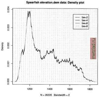Figure 13.7. R/GRASS: Density plot of Spearfish elevation.dem data

see a local over-representation of the contours compared to the interpolated values (depending on interpolation method, see Jacoby, 1997:23pp for details).

Note that NA values are not permitted in the R density function, therefore we mask them on the fly. The legend has to be placed by mouse into the graph, the locator() function silently waits for a click of the middle mouse button:

plot(density(na.omit(elev.f$z), bw=2), col= black ,

main= Spearfish elevation.dem data: Density plot ) lines(density(na.omit(elev.f$z), bw=4), col= green ) lines(density(na.omit(elev.f$z), bw=6), col= brown ) lines(density(na.omit(elev.f$z), bw=8), col= blue ) for (i in seq(1000, 1900, 20)) lines (c (i,i), c(0,0.015), lty=2,

col= grey )

legenddocator 0 , legend=c ( bw=2 , bw=4 , bw=6 , bw=8 ), col=c( black , green , brown , blue ), lty=l)

Instead of the locator() function you can also specify x,y coordinates related to the current coordinates ranges. In our example, you may specify 1600, 0.004 instead of locator(). The graph (see Figure 13.7) shows only slight artifacts up to a kernel bandwidth of 4 meters. These methods may

You can see the complete list of variables in the utm.maas object with str(utm.maas). The second plot() command plots only a subset of all variables. As we want to analyze the zinc contamination, we focus on these

be interesting to compare results from different interpolation methods as described in Section 6.4.3 or to verify unknown interpolated data.

13.2.2 Maas river bank soils data analysis

When analyzing spatial data taken at various sample locations, we may be interested in predicting values in unsampled areas. With variogram modeling and kriging we can generate raster surfaces from point spatial data. GRASS does not include functional modules for analysis of variograms, but R provides extended capabilities. See Section 7.3.8 for a short discussion on geostatis-tics, kriging and splines. The next examples cover basic data analysis while variogram analysis and kriging are not presented due to the complexity of the topic. The R libraries fields and geoR, partly also the R/GRASS interface provide the relevant functionality and examples.

To do the following examples we must run R from inside GRASS. This time we will use the data set which is stored in the R/GRASS interface (and which

was the base for the GRASS Maas LOCATION).

Maas soil data analysis. To set the environment, start GRASS with the maas LOCATION and R within GRASS. Note that you can always use help(function) to read a functions help page and example(function) to run the examples provided for that function. This will also show examples explained in this section as they are based on the interface documentation. Inside R first load the environment and, in this case only for plotting purposes, the library geoR (Ribeiro and Diggle, 1999, Ribeiro and Diggle, 2001, see also online10) which provides numerous geostatistical functions:

grass53 /usr/local/share/grassdata/maas/userl/

g.region -dp

library(GRASS) G <- gmeta() library(geoR)

Next load the maas data set (this time directly the built-in data). The Maas data set contains numerous variables. You can plot all variables against each other (compare Burrough and McDonnell, 1998:112):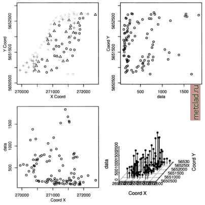

Figure 13.8. R/GRASS: Maas river bank zinc contamination data. Upper left: zinc contaminations quantile plot; upper right: zinc data against y coordinates; lower left: zinc data against x coordinates; lower right: 3D scatterplot

data now. We generate an empty data frame, in which we store the coordinate pairs as matrix and the related zinc (Zn) concentrations in the data variable: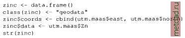

The function class() is used to store the class information in the object. The plot() function uses this information to invoke the standard data plot as implemented in geoR package. As we have compounded several variables into the zinc data object, we can plot numerous graphs right away, according to the definitions in underlying functions of plot.geodataO :