OPEN SOURCE GIS Spearfish soil data: Total Area (ha) - Mean elevation (m)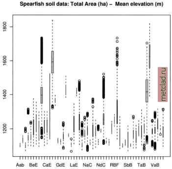

Figure 13.4. R/GRASS: Boxplot of soil type distribution against altitude in Spearfish region (calculated at 100 m raster resolution). The box sizes are representing the area sizes

colnames(soiltable) <-c( Average Height (m) , Tot. Area (ha)

Min. Height (m) , Max. Height (m)

soilareas

dim(soilareas)

boxplot(spearfish$dem spearfish$soils.f,

width=soilareas[2:55], col= gray , horizontal=TRUE) title( Spearfish soil data: Total Area (ha) -

Mean elevation (m) )

soiltable soil.h.range

The boxplot (see Figure 13.4) does not display all soil names due to the space limitations. When directly calling object soiltable in the terminal window the values table is printed into the terminal. In soil.h.range the elevation ranges per soil name are stored. While some soil types are found in a wider elevation range (e.g. VBF, Vanocker-Citadel association, from 1117 m - 1705 m altitude), others are restricted to much narrower range (e.g. NaC, Nevee silt loam, from 1072 m - 1292 m altitude). Boxplots such as above help to show more about the empirical distributions of cell values.

Analyzing interpolated maps. The empirical cumulative distribution function (ECDF) can be useful for identification of a bias towards contours in interpolated DEMs. It is also known as hypsometric integral. After generating a data frame of the input raster map, the ECDF function can be plotted directly. To improve legibility, we use a for() loop to draw lines in the range of the elevation. After starting R and loading the R/GRASS interface, we run:

library (stepfun)

elev <- rast.get(G, elevation.dem )

elev.f <- data.frame(east (G), nortli (G), elev$elevation.dem) names(elev.f) <- c( x , y , z ) summary(elev.f)

plot(ecdf(elev.f$z), verticals=T, do.points=F,

xlab= elevation , main=NULL) for (i in seq(1000, 1900, 20)) lines (c (i,i), c(0,l), lty=2,

col= red2 )

title( Spearfish elevation.dem data: ECDF plot )

As shown in Figure 13.5 the plot looks very smooth. This indicates that the Spearfish raster map elevation.dem does not have waves along contours.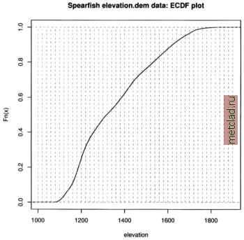

Figure 13.5. R/GRASS: Empirical cumulative distribution function (ECDF) plot to identify interpolation artifacts in Spearfish integer elevation.dem map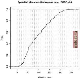

Figure 13.6. R/GRASS: Empirical cumulative distribution function (ECDF) plot to identify interpolation artifacts in Spearfish reclassified elevation.dted map

For comparison we can do the same analysis with the elevation.dted, a map which was reclassified from the original elevation data:

dted <- rast.get (G, elevation.dted )

dted.f <- data.frame (east (G), north(G), dted$elevation.dted)

names(dted.f) <- c( x , y , z )

plot (ecdf (dted.f$z), verticals=T, do.points=F,

xlab= elevation class , main=NULL) for (i in seq(0, 300, 10)) lines (c (i,i), c(0,l), lty=2,

col= red2 )

title( Spearfish elevation.dted reclass data: ECDF plot )

As expected, stairs are visible in the ECDF plot (see Figure 13.6). They are the result of the reclassification of the original elevation map to a reclassed map.

An additional useful tool for analysis of interpolation artifacts is the density plot over elevation (smoothed histogram). The function density() computes kernel density estimates with the given kernel (default: Gaussian) and given bandwidth. If the DEM was interpolated from contour lines, we can probably