To see all data objects which are currently loaded into R, use the ls() function. Next we want to plot the map stored in object soils.ph.frame:

A new window opens with the pH values map displayed. The map colors may differ from GRASS display, but they can be adjusted. The object soils.ph.frame is now prepared for further analysis. Next we can calculate the cubic trend surface with function surf.lsO (Venables and Ripley, 2002). The function does not accept no-data (NA) values, so we have to mask all NAs by na.omitO function. The functions to fit the trend surface through the data points are provided by spatial package which we have to load first:

library(spatial)

ph.ctrend <- surf.ls(3, na.omit(soils.ph.frame)) summary(ph.ctrend)

This function fits a polynomial model to the data set. The parameters for the trend surface modeling function are the degree of polynomial surface (in our case it is 3 for a cubic polynomial) and the data frame with NAs omitted. The calculations require some memory and computational power. The generated trend surface model is then stored into the object ph.ctrend. From this model the trend surface map is evaluated by function trmat.GO . The resulting map can be visualized either as contour lines (function contour.GO) or as solid surface (plot() function). To shorten commands, we evaluate the trend surface on the fly directly within the plot() function which draws the surface into the R graphics window:

plot(G, trmat.G(G, ph.ctrend), col=terrain.colors(20))

Another option is to store the trend surface map into its own object and plot it later (as a solid surface or labeled contour lines):

trendSurf <- trmat.G(G, ph.ctrend)

plot(G, trendSurf, col = terrain.colors (20))

contour.G(G, trendSurf)

title ( Cubic trend surface of pH values in Spearfish region )

It is possible to redirect the R graphical output into a file. For example, to export plots into a Postscript file (function postscript() ), use: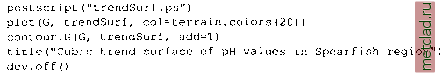

OPEN SOURCE GIS Cubic trend surface of pH values in Spearfish region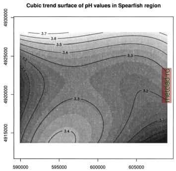

Figure 13.3. R/GRASS: Cubic trend surface of pH values in Spearfish region (calculated at 100 m raster resolution)

The additional parameter add=T for the function contour.G() overlays the contour lines over the previous map plot. The dev.offO call writes the requested postscript file. Other devices are pdf(), pictex(), x11() (the screen), png(), xfig() and jpeg() .To generate EPS (Encapsulated PostScript) files compatible for integration into other documents, e.g. into LaTeX, you may want to use the function dev.copy2eps(). The cubic trend surface from Spearfish pH values is shown in Figure 13.3.

Sometimes it may be necessary to free some memory, so we want to remove objects:

Note that removing objects before leaving the R program is not needed (we just wanted to show how to do it in general). The function history() works similarly as the UNIX history command: It displays all commands used in the current R session.

Working with reclassified raster maps. In this sample session we want to find the average elevation of each of the Spearfish soil classes and the area occupied by each of the classes in hectares. In GRASS, this is done by creating a reclassed map layer in r.average, which assigns mean values to the category labels, and r.report to access the results: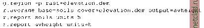

Remember that documentation material, such as soil names explanations for the Spearfish soils map, can be found on the GRASS Web site ( sample data section).

To answer the same question in R using the R/GRASS interface, we import the two required maps into R, soils as factor map (classes), and elevation.dem as a numeric vector: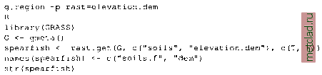

While the soil classes are imported with category label support, the labels for the elevation are omitted. Again we rename the variables for convenience. R provides the tapply() function which lets us apply the declared function mean() to the subsets of the first argument grouped by the second, giving the results we need. The count of cells by land use type are given by table(), which we use to convert square meters to hectares using the metadata on cell resolution. Finally, as an advantage over GRASS functionality, we can construct a boxplot of elevation by soil unit, making box width proportional to the number of cells in each land use class using the table soilareas (note that we drop the areas filled with NA values by subsetting to the row range 2 - 55 with soilareas[2:55]). We get the number of rows, number the of soil types (55 including the no-data area) from the dim() function which returns number of rows and columns:

soil.h.mean <- tapply(spearfish$dem, spearfish$soils.f, mean) soil.h.min <- tapply(spearfish$dem, spearfish$soils.f, min) soil.h.max <- tapply(spearfish$dem, spearfish$soils.f, max) soil.h.range <- tapply(spearfish$dem, spearfish$soils.f, range) soilareas table (spearfish$soils.f)*((G$ewres*G$nsres)/10000) soiltable <- cbind(soil.h.mean,soilareas,soil.h.min,soil.h.max)