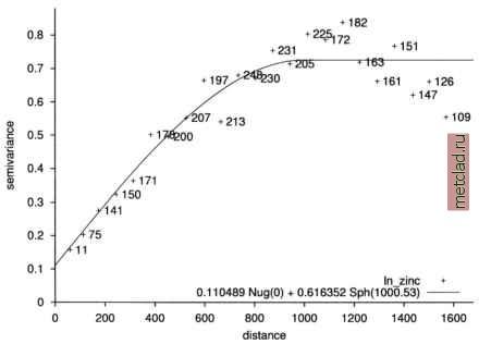Figure 13.1. gstat/GRASS: Semivariogram of zinc contaminations of the Maas river bank soil samples (variogram model: WLS, weights n(h))

After reaching the menu you can move around with cursor keys. Now choose the variable ln zinc (logarithmic transformed zinc concentrations) with <ENTER>. Set the cutoff (lag distance) to 1600 and width to 70. Then select for fit methods WLS, weights n(h) (WLS is weighted least squares, other methods are also available). Now the variogram model will be fitted when hitting the <TAB> key or selecting show plot <Tab>. The resulting semivariogram is shown in Figure 13.1.

Zinc contamination kriging example. In the next example (adapted from Pebesma, 2001:12) we will include a raster MASK and perform ordinary krig-ing prediction from the zinc data. This will result in a raster surface map with predicted distributed zinc contaminations and the predicted kriging error. The gstat instructions file looks as follows (store it as file gstat.maas2.zn):

# ordinary kriging prediction #

data (zinc): zinc, x=l, y=2, v=l;

variogram(zinc): 0.0717 Nug(O) + 0.564 Sph(917.8); mask: maasmask;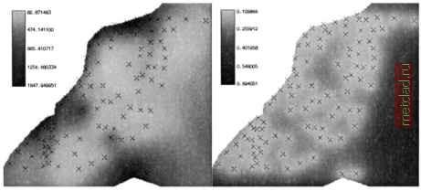

Figure 13.2. gstat/GRASS: Ordinary kriging prediction of zinc contaminations on the Maas river bank. Left: predicted zinc contaminations [ppm], right: prediction error

predictions(zinc): zinc pr.map; variances(zinc): zinc var.map;

In general, output grid maps are always written in the same format as the input mask map. Besides the GRASS format, gstat also supports other GIS formats. Before running the prediction, we have to generate the GRASS raster map maasmask. The Maas LOCATION contains a raster map maasbank which covers the river bank area. We generate the desired binary map from this map, then we run the kriging prediction: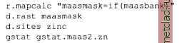

During calculations the program will report similar user messages:

gstat: Linux version 2.4.3 (04 January 2004) Copyright (C) 1992, 2004 Edzer J. Pebesma using Marsaglias random number generator data(zinc): gisrc: [/home/neteler/.grassrcS] GRASS site list zinc: 0 cat, 2 dim, 0 str, 1 dbl. gstat/grass: 98 sites read successfully.

zinc (GRASS site list)

attribute: col[l] [x:] x l

n: 98 [y:l y 2

sample mean: 481.031 sample std. [using ordinary Icriging] ncols 259 nrows 232

initializing maps ..

[ 269870, 272460]

[5 . б50б1е + 0 6,5.б52 93е + 06] 398 . 808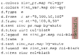

The result is shown in Figure 13.2. For further details and examples please refer to the gstat documents.

13.2. SPATIAL DATA ANALYSIS WITH GRASS AND R

The R data analysis programming language and environment (Ihaka and Gentleman, 1996, available from Internet7), a dialect of S (Becker, 1988), is an extensible system which can be connected directly to GRASS. R consists of a base package and extensions that can be downloaded from the project Web site. A regular newsletter informs about recent changes and improvements.8 Besides classical methods, graphical and modern statistical techniques are implemented in the base R library and supplementary packages. Latter comprise packages for point pattern analysis, geostatistics, exploratory spatial data analysis and spatial econometrics. While R is a general data analysis environment, it has been extensively used for modeling and simulation. Through the R/GRASS interface (Bivand, 2000, Bivand and Gebhardt, 2000, Bivand and Neteler, 2000, Furlanello et al., 2003) the geospatial analysis capabilities of GRASS are substantially improved.

For the integration of R into GRASS you need to run R from the GRASS shell environment. The interface dynamically loads compiled GIS library functions into the R executable environment. The GRASS metadata about the LOCATIONS regional extent and raster resolution are transferred to R. In interpreted mode, when the interface installation was not compiled with the GRASS GIS library, this is taken from g.region. The R/GRASS interface

CREATING SUPPORT FILES FOR zinc pr.map CREATING SUPPORT FILES FOR zinc var.map 100% done

Two new raster maps have been generated, which contain the predicted zinc distribution (zinc pr.map) and the distributed error (zinc var.map). Using d.frame we can display both maps side-by-side in the GRASS monitor: