
|
|
|
|
Главная --> Промиздат --> Map principle The displayed map shows that almost each field needs two or more grassways, (Figure 12.6). And the report provides us with an estimate of over 1 acre for grassed area within the fields. Net erosion and deposition modeling using flow divergence. Our previous examples involving erosion processes (both for Spearfish and for grassways) focused on soil detachment. However, the detached soil can be deposited relatively close to the source without causing pollution problems in the streams. Simulating net erosion and deposition under spatially variable topographic and land cover conditions is a complex task and requires external simulation tools. However, a simplified estimate of erosion and deposition pattern can be obtained relatively easily using the concept of flow divergence. 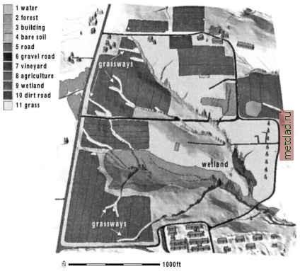 Figure 12.6. Proposed grassways viewed as dense sites draped over DEM with the current land cover displayed as a color map. The DEM has buildings and sediment flow potential added to elevation to enhance the understanding of relation between flow and land use in the watershed The Unit Stream Power Based Erosion/Deposition model (USPED, Mitasova et al., 2001) estimates a simplified case of erosion/deposition using the idea originally proposed by Moore and Burch, 1986. It combines the RUSLE parameters and upslope contributing area per unit width A to estimate the sediment flow T: The net erosion/deposition D is then computed as a divergence of sediment flow: where ain degrees is the aspect of the terrain surface (direction of flow). The exponents m,n control the relative influence of water and slope terms and reflect the impact of different types of flow. The typical range of values is m = 1.0 - 1.6, n = 1.0 - 1.3, with the higher values reflecting the pattern for prevailing rill erosion with more turbulent flow when erosion sharply increases with the amount of water. Lower exponent values close to m = n = 1 better reflect the pattern of compounded, long term impact of both rill and sheet erosion and averaging over a long term sequence of large and small events. Caution should be used when interpreting the results from USPED, because the RUSLE parameters were developed for simple plane fields and detachment limited erosion. We have already computed slope, aspect, and flow accumulation map layers. We now need to use them to compute the estimate of sediment flow and its divergence, while taking into account variability in land cover. First, we create a C factor map layer by recoding the land cover map, where we will recode the forest to 0.0005, grass to 0.005, agricultural fields, including the grapes and gravel road to 0.5, dirt road to 0.7, and bare soil to 0.8: 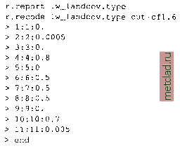 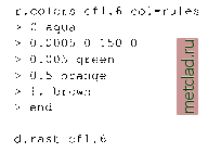 To account for variability in soils and to incorporate the relative impact of rainfall, we also include the K and R = 270 factors. We use the topographic sediment flow map sedflow.6 (m = n = 1) and compute the net erosion/deposition using the equation 12.4: 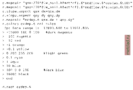 Red-orange-yellow areas show erosion and blue shades represent deposition. Obviously, concentrated flow appears to be the largest source of sediment pollution which we have addressed in the previous paragraph. About one magnitude lower, but still very high erosion is predicted in the agricultural fields, if they were managed as a single, homogeneous area which can be bare for several weeks or even months. We can also see that not all of the eroded soil will be transported out of the fields. A substantial portion can be deposited directly in the field concave areas and an additional amount is deposited on the border of the field, where water is slowed down by grass. To improve the stability of the fields, they have been divided into subsections which are planted with
|