inputs (see Section 5.4.5, the manual page for r.sun and Appendix B.4 for more details on this module). If the growing season for a specific crop is between March 15 and October 15, we can use a shell script (see Chapter 11) to compute a sum of daily global radiation for this period of the year:

min/sh

echo Enter elevation map: read elev

g.copy rast=$eev,SOLelev echo Enter slope map: read si

g.copy rast=$s£,SOLslope echo Enter aspect map: read asp

g.copy rast=$asp,SOLaspect

echo Enter Latitude of given region: read lat

i=75

laslday=288

generate an empty map for global radiation: r.mapcalc global. rad=0

while [ $1 -le $£astday ] do

# generate map names convenient for xganim and r.out.mpeg: DAY=echo $i I awk Iprintf %03i , $1)

echo Computing radiation for day $DAY. . . r.sun elevin=SOLelev aspin=SOLaspect slopein=SOLslopc\

lat= Slat day= $i \

beam.rad=b.rad.$DAY diff-rad=d.rad.$DAY\ ren rad=r rad.$DAY

#add to (celt-wise) global energy:

r.mapcalc global. rad=global. rad + b rad.$DAY +\

d rad.$DAY + r rad.5DAY r.timestamp b rad.$DAY date= $i days r.colors b rad.$DAY col=gyr r.timestamp d rad.$DAY date= $i days r.colors d rad.$DAY col=gyr r.timestamp r rad.$DAY date= $i days r.colors r-rad.$DAY col=gyr

i=expr $i + 1 done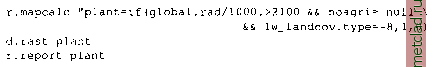

We can use r. report to find how large is the area that is suitable for our plant. The resulting time series of radiation maps (e.g. b rad.075 through b rad.2 8 8) can be animated in xganim to get a better insight into evolution of solar radiation pattern:

xganim viewl= b rad.*

The module also allows us to display several maps simultaneously as time

series:

To animate the result in 3D as a color draped over the DEM along with the vector map layer representing the land use polygons, you can use nviz scripting capabilities with the file sequencing tool (see Section 8.2.3 and nviz tutorial for more details).

Planning conservation measures using estimate of sediment flow. The

flow accumulation map flowacc.6 indicates a significant potential for negative impact of concentrated flow, which can cause formation of gullies and transport of sediment and pollutants through protective stream buffers. One of the common practices to mitigate the possible impact of concentrated flow are grassed waterways.

We can use a simple combination of topographic analysis and map algebra to identify the areas which may need protection by grassed waterways. This type of management practice requires installation of a grassed path in those areas which have concentrated flow and which are without protective vegetation during certain time of year (for example agricultural fields). First, we find the high risk areas by computing a topographic index for sediment flow, which combines the upslope area (flow accumulation multiplied by resolution) with slope (we have computed both layers in the Section 12.2.2):

icleanup:

g.remove rast=SOLelev,SOLaspect,SOLslope echo Finished.

The module outputs all three components of global radiation separately, so we need to add them to get the global radiation. We then use map algebra to find the areas within the agricultural fields where this value exceeds our given threshold, while excluding the areas which were identified as unsuitable for growing crops in the previous paragraph:

r.mapcalc sedflow.6=flowacc.6*6*sin(si.6tl0) r.colors sedflow.6 col=rules fp: Data range is 0.00 to 2 6 663.21484375

> 0 200 255 200

> 10 yellow

> 50 orange

> 100 red

> 500 magenta

> 30000 violet

> end

d.rast sedflow.6

We have assigned a special color table to the new map highlighting the high sediment flow areas. We now extract those areas where the value of the sediment flow index is greater than 50 and display the result over the land use map: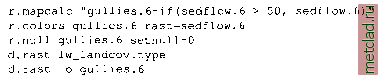

We can see that we have a high risk area in almost every field. To create a map of proposed grassways we use map algebra to extract the potential gullies in the areas with agricultural land, grapes, and bare soil (categories 8, 4, 7):

r.mapcalc grassway.6=if{(lw landcov.type ==8 II \

lw landcov.type ==4 M \ lw landcov.type == 7) && \ gullies.6, 1)

r.null grassway.6 setnull=0

r.colors grassway.6 col=rules

> 1 green

> end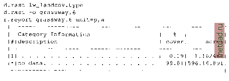