Note that you may get slightly different numbers for Isfactor.lSm because your DEM will be re-computed from a different set of random points than the one used in this book. The results show that the mean LS factor is lower for the 30 m resolution, which was expected from the visual comparison. The reinterpolation of the DEM to 15 m resolution brings the result closer to the values derived from the new, more accurate 10 m resolution DEM. The difference in range is much larger; however, displaying the cells with values over 180 by d.rast Isfactor.lSm val=180-280 reveals that the higher values are only present in very few cells (41 out of over 1 million). These are mostly due to the fact that smoothing removed some of the smaller pits and the flowlines are generally longer. To quantify the visible differences in the extent of LS = 0.0 values and assess their impact, we extract them from the lsfactor.30m, Isfactor.lSm, and Isfactor.lOm map layers using r.mapcalc and compute their proportion with r.report:

g.region rast=lsfactor.30m

r.mapcalc IsfacO.30m=if(Isfactor.30m==0.ООО,0,1) r.report -n IsfacO.30m unit=p [...]

0.....................I 20.031

HI.....................I 79.971

g.region rast=lsfactor.15m

r.mapcalc IsfacO.15m=if(Isfactor.15m==0.000, 0, 1) r.report -n IsfacO.15m unit=p [...]

jOI.....................I 3.991

111.....................I 96.011

g.region rast=lsfactor.10m

r.mapcalc IsfacO.10m=if(Isfactor.10m==0.000,0,1) r.report -n IsfacO.10m unit=p [ . . . ]

101.....................I 2.711

111.....................I 97.291

The new binary layers have 0 in those areas where the LS = 0.000 (with floating point accuracy) and 1 everywhere else. You can see that there is a significant difference in the spatial extent of zero areas between the original map (20.03% !) and the re-interpolated map (3.99%). Again, comparison with the percent area with LS = 0.000 for lsfactor.10m (2.71%) demonstrates that reinter-polation to 15m resolution brings the results much closer to the ones obtained from more accurate 10m resolution DEM. You can also run d.histogram for lsfactor.1Sm and lsfactor.30m and see how the lower values of erosion are lumped into the zero LS factor when the original data were used. This is the impact of insufficient vertical resolution, which causes the topography in low

slope areas being represented by plateaus with zero slope. Using the result directly derived from the original DEM would have significantly underestimated the spatial extent of area with topographic potential for erosion; therefore, we will continue our computation and analysis using the Isfactor.lSm map layer.

If you display the LS values higher than 40.0 using:

d.rast Isfactor.lSm val=40-400

you will see that these high values cover only very small, narrow areas with concentrated flow. In these areas (hollows, upland valleys), values are substantially higher than those typical for the traditional field application of USLE, because they indicate a risk for gully erosion, not modeled by traditional USLE. You can also see that the mountains have the highest topographic risk of erosion due to steep slopes and a high density of concentrated flow areas. However, the mountains have also the largest proportion of forest, so we will now compute the full equation, including the cover factor C, to see how much the forest cover compensates for the high topographic risk.

12.1.2 Estimating R, K, and C factors

The R factor is not spatially variable in our study area and we can use a constant R = 65 (you can find the values in any USLE handbook or a related textbook such as Haan et al., 1994). The soil erodibility factor K is already included in the Spearfish data set as a raster map soils.Kf actor. You can check its values by running r.report soils.Kfactor and you will see that the K values are stored as category labels ranging from 0.10 to 0.43 for categories 1 through 8.

The C factor is based on land cover. It can be derived from the 100 m resolution vegetation map vegcover by editing the category labels. A more detailed C factor map can be created from the new 30 m resolution land cover map. It has larger number of classes, so using r.recode will be more efficient. The C-factor values for different types of land cover can be obtained from literature (Haan et al., 1994).

When using the category approach (more typical for GRASS4.*, when only integer values were allowed for raster map layers), copy the map vegcover to cfactor.lQQ and modify the category labels:

g.copy vegcover,cfactor.100m r.support

Enter name of raster file for which you will create/modify support files [. . .1

> cfactor.lOOm

Edit the header for [cfactor.lOOm]? n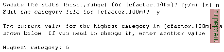

Do not change the number of categories and proceed to the next step using <ESC> <ENTER>. You can now change the TITLE and replace the category labels representing the vegetation by the C factor values: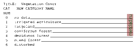

Retype the TITLE and labels to: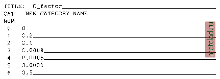

Leave this screen with <ESC><ENTER>, and move on using <ENTER> on all remaining questions. Now you have a C factor map with raster cells containing the value of the category number and with each category labeled with C factor. The P factor is not available, so we can assign it a value of 1.0 and ignore it in our further computations.

Recently, USGS started to provide seamless National Land Cover Dataset on-line, so it was possible to download a much more detailed, 30 m resolution land cover map for Spearfish. We have included it in the Spearfish data set as a raster map layer landcover.SQm. You can use this map to create a refined C factor layer by receding the land cover classes to C factor values as follows (run r.report to see the land cover associated with each class):